
In complex chemical reactions, especially those involving reactive intermediates or radicals, solving rate equations can be difficult. To simplify things, chemists often use the steady state approximation (SSA)—a powerful tool in chemical kinetics. This method assumes that the concentration of short-lived intermediates remains relatively constant over time. In this article, you’ll learn what the steady state approximation is, how to apply it, its key formula, and how it helps in solving real reaction mechanisms.
If you’re unsure how to apply the steady state approximation in reaction kinetics, Eureka Technical Q&A connects you with chemistry professionals who can walk you through the assumptions, derivations, and real-world applications—making tough concepts easier to grasp and use confidently.

What Is the Steady State Approximation?
The steady state approximation is an approach in chemical kinetics that assumes the rate of change of an intermediate’s concentration is zero after an initial transient period. In other words, intermediates are formed and consumed so rapidly that their concentrations remain nearly constant during the reaction.
The steady-state approximation involves assuming that the system has reached a state where the concentrations or values of certain variables no longer change over time. This is based on the idea that the system has sufficient time to adjust to any disturbances, and as a result, the net rates of production and consumption of certain species or variables are equal, leading to a constant value.
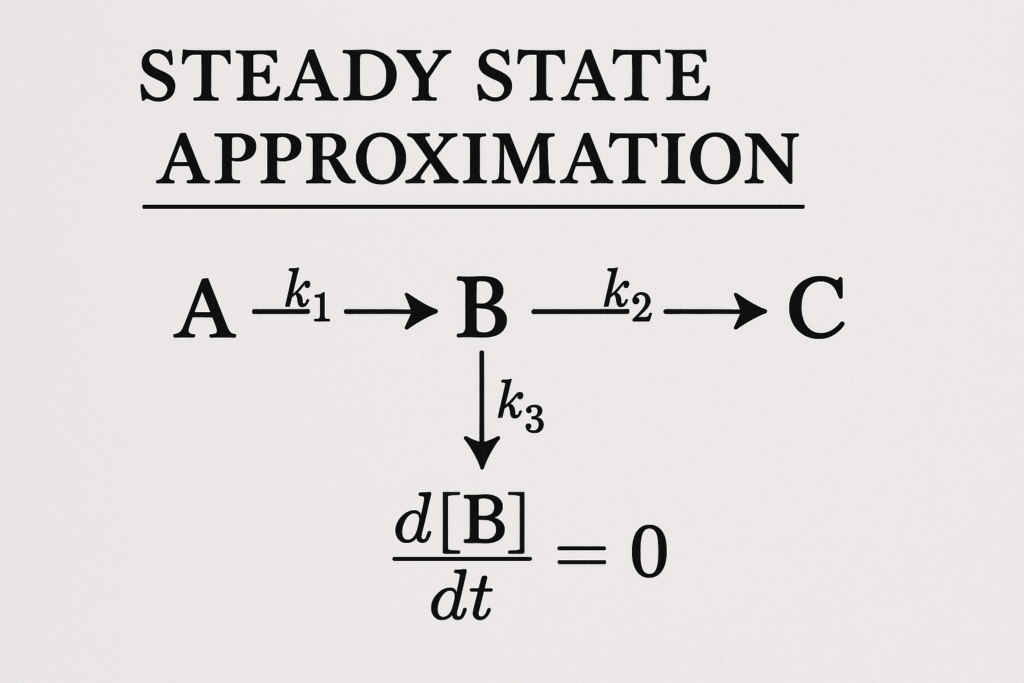
Key Concept:
If [I] is the concentration of an intermediate:
d[I]/dt ≈ 0
This simplifies the rate equations and allows us to derive expressions for the overall rate of reaction in terms of reactants only.
When Is It Used?
Steady state approximation is commonly applied when:
- The mechanism involves short-lived intermediates
- The intermediate is present in very low concentration
- The intermediate is formed and consumed in consecutive steps
It is often used in enzyme kinetics, chain reactions, photochemistry, and reaction mechanisms involving radicals.
| Product/Project | Technical Outcomes | Application Scenarios |
|---|---|---|
| ACS Reaction Mechanism Generator American Chemical Society | Implements quasi-steady-state approximation for simplifying complex reaction-diffusion equations, improving computational efficiency. | Modeling of complex chemical reactions in atmospheric chemistry and combustion systems. |
| MATLAB Chemical Engineering Toolbox MathWorks | Incorporates steady-state approximation algorithms for solving reaction-diffusion problems with improved accuracy. | Analysis of chemical processes in pharmaceutical manufacturing and environmental engineering. |
How the Steady State Approximation Works
Step-by-Step Approach:
Identify the System and Its Processes
Start by selecting the system you want to analyze. It could be a chemical reaction network, a physical system, or a dynamic process. Next, define the inputs, outputs, and internal interactions that shape the system’s behavior.
Define Key Variables and Parameters
List the essential variables and parameters that influence the system. These may include concentrations, temperatures, flow rates, or pressures. Choose only the quantities that significantly affect how the system evolves over time.
Establish Governing Equations
Create mathematical equations that describe the system’s dynamics. Use differential equations, algebraic expressions, or any format that accurately models the changes within the system. These equations form the foundation for further analysis.
Assume Long-Term Equilibrium Conditions
To simplify the analysis, assume the system reaches a point where its properties no longer change with time. This equilibrium assumption helps focus on the long-term behavior rather than short-term fluctuations.
Simplify the Equations
Now, apply the equilibrium condition to your equations. Set time derivatives to zero to remove the time-dependent terms. This step transforms complex dynamic equations into simpler algebraic forms.
Solve for the Equilibrium Values
Solve the simplified equations to find constant values for your system’s variables. These represent the system’s stable state when no further changes occur. Use standard algebraic techniques to find accurate results.
Interpret the Outcomes
Once you have the equilibrium values, relate them back to the system. Determine what they reveal about reactant levels, energy flow, or other performance indicators. This helps you understand how the system operates under stable conditions.
Validate the Equilibrium Assumption
Before using the results, confirm that your system actually reaches a stable state over time. Run simulations, perform experiments, or use analytical checks to support your assumption and verify your conclusions.
Apply the Results for System Analysis
Use the equilibrium findings to guide decisions, predict behavior, or improve system design. These insights are especially useful when assessing long-term outcomes or optimizing system performance.
Recognize Limitations and Explore Improvements
Finally, consider where your analysis might fall short. Some systems show multiple equilibrium points or take a long time to stabilize. You may need to refine your model to include transient effects or system-specific complexities.
Example: Unimolecular Reaction via an Intermediate
Mechanism:
- A → I (rate constant k₁)
- I → P (rate constant k₂)
I is the intermediate.
Applying SSA:
Assume d[I]/dt = 0
So,
Rate of formation of I = Rate of consumption of I
k₁[A] = k₂[I] → [I] = k₁[A]/k₂
Overall rate of product formation:
Rate = k₂[I] = (k₁k₂[A])/k₂ = k₁[A]
In this case, the rate simplifies back to a first-order rate law.
Example: Chain Reaction (H₂ + Br₂ Reaction)
Mechanism:
- Br₂ → 2Br· (initiation)
- Br· + H₂ → HBr + H· (propagation)
- H· + Br₂ → HBr + Br· (propagation)
Intermediates: Br· and H·
Using SSA on both Br· and H· allows us to derive the full rate law in terms of H₂ and Br₂ only, rather than trying to track reactive radical concentrations directly.
Formula Summary
For intermediate I in a two-step mechanism:
- Formation: A → I (rate = k₁[A])
- Consumption: I → P (rate = k₂[I])
Apply SSA:
d[I]/dt ≈ 0 → k₁[A] = k₂[I] → [I] = k₁[A]/k₂
Overall rate:
Rate = k₂[I] = k₁[A]
This simplification helps avoid solving complex differential equations.
Pros and Limitations
Advantages:
- Makes complex rate equations manageable
- Useful for multi-step reactions
- Applicable to radical and enzymatic processes
Limitations:
- Assumes intermediates are in low concentration
- Not valid during the early (induction) phase of the reaction
- May not be accurate for all mechanisms—especially if intermediate builds up
FAQs
Is steady state approximation the same as equilibrium approximation?
No. The steady state approximation assumes a constant concentration of intermediates, while the equilibrium approximation assumes rapid equilibrium in a reversible step.
Can you use SSA for all intermediates?
No. It’s only valid when intermediates are short-lived and consumed quickly after being formed.
Is SSA used in enzyme kinetics?
Yes. It’s the basis of the Michaelis-Menten equation, where the enzyme-substrate complex is treated as being in a steady state.
Does SSA work in reversible reactions?
It can, but you must account for both forward and reverse rates when writing the steady state expression.
Conclusion
The steady state approximation is a vital method in chemical kinetics for simplifying rate laws in reactions with unstable intermediates. By assuming that intermediate concentrations remain constant, chemists can derive rate laws that are easier to work with and understand. Whether in enzyme kinetics, radical chemistry, or multi-step mechanisms, steady state helps bridge complex reaction steps into clear, solvable models.
To get detailed scientific explanations of Steady State Approximation, try Patsnap Eureka.