
A multi-terminal traveling wave ranging method for t-junction lines based on the distribution characteristics of fault traveling waves along the line
A technology of traveling wave distance measurement and distribution characteristics, which is applied to the location of faults, detecting faults according to conductor types, and measuring electrical and other directions
Patent Information
- Authority / Receiving Office
- CN · China
- Patent Type
- Patents(China)
- Current Assignee / Owner
- Publication Date
- 2019-07-16
Smart Images
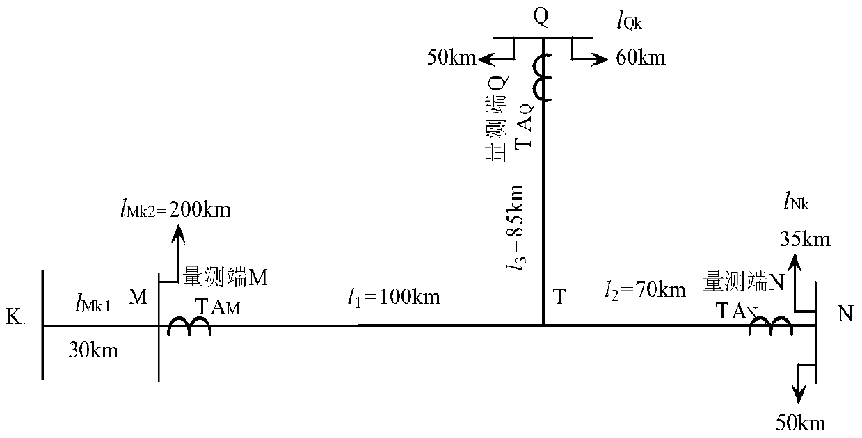
Figure 1 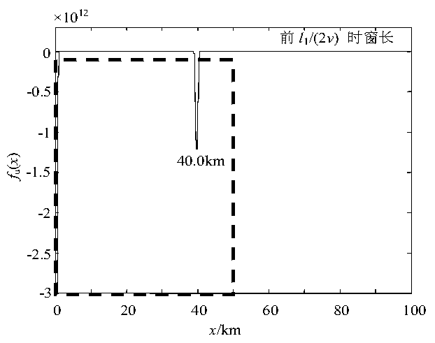
Figure 2 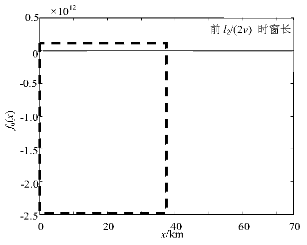
Figure 3
Abstract
Description
technical field
[0001] The invention relates to a multi-terminal traveling wave ranging method of a T-connection line based on the distribution characteristics of fault traveling waves along the line, and belongs to the technical field of electric power system relay protection. Background technique
[0002] The task of fault location is to calculate the fault distance through the measured current, voltage and line impedance parameters at both ends of the line when a fault occurs at a certain point of the line. Generally, there are two main types of transmission line fault location methods, one is the impedance method, which is an algorithm to directly calculate the fault impedance or its percentage; the other is the traveling wave method, which uses the traveling wave of high-frequency fault transient current and voltage etc. to indirectly determine the distance to the fault point.
[0003] Transmission line traveling wave fault location has gone through two stages: early t...
Examples
Embodiment 1
[0106] Embodiment 1: with figure 1 Take the transmission line shown as an example, assuming that the MT branch is 40km away from the M terminal and a phase A ground fault occurs.
[0107] According to step 1 and step 2 in the instruction manual, the ranging function f of the measuring terminal M, measuring terminal N and measuring terminal Q of the ranging function is obtained Mu (x), f Nu (x) and f Qu (x). Get f according to step 3 Mu =[40.0],f Nu = φ (represents the empty set), f Qu =[39.8]. by f Nu = φ, it can be seen that the fault is not located in the NT branch, then use the data of the measuring terminal N to calculate [t 0 ,t 0 +l 3 / (2v)] The ranging function in the time window is along l 3 The mutation distribution f' in the range of line length Nu =[40.0]. It can be seen that x M1 =x' N1 ≈x Q1 , and sgn(x M1 )&sgn(x N )=0, sgn(x M )&sgn(xQ )=0, and sgn(x N )&sgn(x Q )=1. It can be seen that the fault is located in the MT branch, and the distanc...
Embodiment 2
[0108] Embodiment 2: with figure 1 The transmission line shown is taken as an example, assuming that the NT branch is 25km away from the T node, and a phase A ground fault occurs.
[0109] According to step 1 and step 2 in the instruction manual, the ranging function f of the measuring terminal M, measuring terminal N and measuring terminal Q of the ranging function is obtained Mu (x), f Nu (x) and f Qu (x). Get f according to step 3 Mu =[24.7 44.9],f Nu =[24.7], f Qu =[24.7], it can be seen that x M1 =x N1 =x Q1 , and sgn(x M )&sgn(x N )=0, sgn(x M )&sgn(x Q )=1, and sgn(x N )&sgn(x Q )=0. It can be seen that the fault is located in the NT branch, and the distance from the J node is 24.7km.
Embodiment 3
[0110] Embodiment 3: with figure 1 Take the transmission line shown as an example, assuming that the phase A ground fault occurs at the point where the QT branch is 20km away from the T node.
[0111] According to step 1 and step 2 in the instruction manual, the ranging function f of the measuring terminal M, measuring terminal N and measuring terminal Q of the ranging function is obtained Mu (x), f Nu (x) and f Qu (x). Get f according to step 3 Mu =[20.0],f Nu =[20.0],f Qu =[20.0], it can be seen that x M1 =x N1 =x Q1 , and sgn(x M )&sgn(x N )=1, sgn(x M )&sgn(x Q )=0, and sgn(x N )&sgn(x Q )=0. It can be seen that the fault is located in the QT branch and is 20.0km away from the J node.