
Aero-engine model optimization iteration solving method based on LM algorithm and quasi-Newton method
By combining the Levenberg-Marquardt algorithm and the quasi-Newtonian method, the problem of slow solution speed and insufficient accuracy of aero engine models is solved, and the rapid and accurate solution of model equations is achieved, and the optimization speed and accuracy are improved.
Patent Information
- Application Number
- CN202411533677.1
- Authority / Receiving Office
- CN · China
- Patent Type
- Applications(China)
- Current Assignee / Owner
- Filing Date
- 2024-10-30
- Publication Date
- 2025-02-14
- Estimated Expiration
- Not applicable · inactive patent
AI Technical Summary
When solving aircraft engine models, the prior art has problems such as slow solution speed and insufficient solution accuracy, making it difficult to effectively deal with complex engine models.
The optimization iterative solution method combined with the Levenberg-Marquardt (LM) algorithm and the quasi-Newtonian method is used. By calculating the LM step and two approximate LM steps, the algorithm has four convergence speeds under the local error boundary conditions, and the objective function value is used. The information of f and the first derivative g constructs the curvature approximation of the objective function.
It realizes rapid and accurate solution of model equations, improves the speed and accuracy of linear and nonlinear optimization, and can effectively handle complex aero engine models.
Smart Images
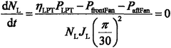
Figure BSA0000299787130000021 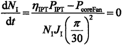
Figure BSA0000299787130000022 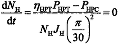
Figure BSA0000299787130000023
Abstract
Description
1. Technical Field
[0001] The present invention relates to the field of iterative solution of various mathematical models, and specifically to iterative solution of aero-engine model matrices, improving the speed and accuracy of linear and nonlinear optimization, and realizing fast and accurate solution of aero-engine models. 2. Background technology
[0002] The component-level model of an aircraft engine is the basis for conducting control research. The common method of building a component-level model is to accurately describe the working mechanism of each component of an aircraft engine based on aerodynamic thermodynamics, and then connect each component in series through a common working equation. The component-level model can be divided into two types: the starting model and the model above the slow speed. Relevant research was carried out abroad in the 1950s, including the early turbojet engine cycle parameter analysis model SPFFDY, which can only perform steady-state calculations for a specific type of aircraft engine, and the turbojet and turbofan engine cycle parameter analysis model CARPFT. In addition, the GENENG and DYGENG programs were successively developed in the 1970s, which improved the accuracy of steady-state simulation and increased the transition state simulation capability. In the mid-to-late 1980s, NASA and the U.S. Department of Defense formally proposed the "Numerical Propulsion System Simulation" (NPSS) program. The program focuses on multidisciplinary simulation, takes into account multi-media coupling simulation during engine operation, establishes a whole-machine simulation system from 0-dimensional simulation to 3-dimensional multidisciplinary dynamic simulation, and develops an object-oriented simulation program NPSS. It has reached a very high technical level. The relevant results have been used in the design optimization process of the GE90 engine, saving $250,000 in design and manufacturing costs for a single engine and greatly reducing the engine development cycle.
[0003] Nonlinear equations are widely present in many fields such as information security and engineering practice. For example, nonlinear finite element problems, nonlinear fracture problems, elastic-plastic problems, economic and nonlinear programming problems can all be attributed to nonlinear equations. The solution of nonlinear equations plays an important role in many computing applications and provides certain theoretical basis and technical support for subsequent research work. However, since there is no specified solution formula for the solution of nonlinear equations, it is difficult to obtain an accurate solution in actual operation. Therefore, it is very meaningful to study the numerical method for solving nonlinear equations.
[0004] In the current aviation engine modeling work, people still generally use Newton's method to solve the model equations. The Newton method has the problem of slow solution speed and insufficient solution accuracy. With the current engine technology, the required models and model solving technology must also be improved accordingly, otherwise the solution accuracy of complex engine models will be low or even impossible to solve. The present invention combines the LM algorithm with the quasi-Newton method and adopts the optimized LM algorithm. The LM step and two approximate LM steps are calculated in each iteration. Under the condition of the local error bound, it is proved that the algorithm has a fourth convergence speed. At the same time, the quasi-Newton algorithm is one of the most effective algorithms for solving unconstrained optimization problems. It improves the linear convergence speed of the first-order method and achieves a local superlinear rate. The computational cost of each iteration is O(d 2 ), rather than Newton's method O(d 3 ). It uses the information of the objective function value f and the first-order derivative g to construct the curvature approximation of the objective function. After multiple iterations of approximate Hessian matrix, there is no need to form the Hessian matrix. The combination of the two algorithms can make the solution of the model equation faster and more accurate. 3. Summary of the invention
[0005] This solution method combines the LM algorithm with the quasi-Newton method, and adopts different solution methods to meet the solution requirements of different models. Its purpose is to solve the problems of inaccurate solution and slow solution speed of some aero-engine models.
[0006] The iterative solution method for optimizing the aero-engine model based on the LM algorithm and the quasi-Newton method mainly includes the establishment and solution of the aero-engine model. The aero-engine model includes the air intake, compressor, combustion chamber, turbine, tail nozzle, and some also include duct ejectors, heat exchangers, and cooling devices. The entire engine model is connected through thermodynamic equations. The airflow flows from the air intake to the tail nozzle along the channel direction. The inlet and outlet parameters of different components are connected by thermodynamic equations, and finally the common working equation of the engine is formed. When modeling, the engine model must also be simplified.
[0007] The engine model used in the present invention is as follows: Figure 1 As shown in the figure, the main components include the front fan, rear fan, core fan, high-pressure compressor, heat exchanger, main combustion chamber, intermediate-pressure turbine, multi-function combustion chamber, low-pressure turbine, afterburner, tail nozzle, etc. The low-pressure rotor is driven by the low-pressure turbine to drive the front fan and the rear fan; the intermediate-pressure rotor is driven by the intermediate-pressure turbine to drive the core fan; the high-pressure rotor is driven by the high-pressure turbine to drive the high-pressure compressor. The mode switching valve is used to control the engine to switch back and forth between turbofan mode and turbojet mode.
[0008] The Levenberg-Marquardt algorithm is an optimization method for solving nonlinear least squares problems, especially for solving problems of the form min x Σ i f i (x) 2 The problem, where f i is a nonlinear function. This algorithm combines the advantages of gradient descent and Gauss-Newton methods. It behaves similar to Gauss-Newton method (fast convergence) when close to the optimal solution, and behaves more like gradient descent method (robustness) when far away from the optimal solution. The core idea is to balance the step size by adjusting a parameter in each iteration, so that the algorithm can automatically select the most appropriate strategy at different stages.
[0009] Quasi-Newton methods are a class of methods used for unconstrained optimization problems, the goal is to find the local minimum of the objective function f(x). This type of method attempts to approximate the Hessian matrix or its inverse matrix to accelerate convergence, while avoiding the complexity and cost of directly calculating the Hessian matrix and its inverse. Common quasi-Newton methods include the DFP (Davidon-Fletcher-Powell) method and the BFGS (Broyden-Fletcher-Goldfarb-Shanno) method. These methods construct an approximate Hessian matrix or its inverse matrix by using the first-order derivative information (gradient) of the function and the information of the previous iterations to determine the search direction.
[0010] Among them, the LM algorithm is particularly suitable for dealing with nonlinear least quadratic problems; while the quasi-Newton method is widely used in various types of unconstrained optimization problems. The LM algorithm balances two different update strategies by adjusting a parameter; the quasi-Newton method focuses on how to effectively estimate the Hessian matrix or its inverse. For certain types of problems (such as nonlinear least squares), the LM algorithm may reach a solution faster than some forms of quasi-Newton methods; but for general unconstrained optimization problems, good quasi-Newton methods (such as BFGS) often provide good performance.
[0011] The equilibrium equation solved by the present invention is:
[0012]
[0013]
[0014]
[0015] The above three equilibrium equations are the equilibrium equations when the engine is working. These equilibrium equations are solved by using an algorithm that combines the LM algorithm with the quasi-Newton method. This algorithm combines the LM algorithm with the quasi-Newton method. This combined algorithm can ensure that the solutions to the equations to be solved are obtained. By using the method of initial value substitution or matrix addition, the equations can be solved faster and more accurately. 4. Description of the drawings
[0016] Figure 1 The engine structure adopted by the present invention is
[0017] Figure 2 Is the model code calling relationship
[0018] Figure 3 Is the meaning of the function
[0019] Figure 4 It is the initial guess search algorithm
[0020] Figure 5 It is the optimization solution comparison 5. Specific implementation methods
[0021] Reference will now be made in detail to specific embodiments of the present invention. Although the present invention will be described in conjunction with specific embodiments, it will be understood that it is not intended to limit the present invention to the described embodiments. On the contrary, it is intended to cover the changes, modifications and equivalents included in the spirit and scope of the present invention as defined by the appended claims. It should be noted that the method steps described herein can all be implemented by any functional block or functional arrangement, and any functional block or functional arrangement can be implemented as a physical entity or a logical entity, or a combination of the two.
[0022] In order to enable those skilled in the art to better understand the present invention, the present invention is further described in detail below in conjunction with the accompanying drawings and specific implementation methods.
[0023] The invention proposes an iterative solution method for optimizing an aero-engine model based on the LM algorithm and the quasi-Newton method, which can be used to solve the variable cycle engine models of various types. Figure 1 Taking the engine model shown in the figure as an example, in the actual modeling process, since the aerodynamic thermodynamic process inside the engine is very complicated, it is very difficult to use a mathematical model to fully describe its working process. Therefore, the engine needs to be simplified before modeling:
[0024] (1) Ignore the effects of component thermal inertia and combustion lag in the combustion chamber;
[0025] (2) The gas is treated in a quasi-one-dimensional flow in the flow path;
[0026] (3) Ignore the effects of Reynolds number and atmospheric humidity on engine performance parameters.
[0027] Following the above rules, we carried out research on engine modeling technology. Based on MATLAB2021b, we wrote a complete engine model function library, which contains a complete engine model, thermodynamic functions, model solving algorithms and user interfaces. The code calling relationship is as follows: Figure 2 As shown, the blue one is the physical model of the component, and the red one is the basic thermodynamic function. The meaning of each function is as follows Figure 3 As shown, the engine components are modeled according to the principles of thermodynamics. At the same time, the model adopts a volumetric model to make the overall modeling of the engine closer to the actual situation and the model more accurate.
[0028] When considering the volume effect, there are 43 equations to be solved, including 7 equilibrium equations and 36 differential equations. The differential equations are solved using the solve function of Matlab. Here we mainly study the solution algorithm of the equilibrium equations, which can be roughly divided into three parts:
[0029] (1) Select an appropriate initial guess.
[0030] (2) Select an efficient iterative algorithm.
[0031] (3) Select an appropriate convergence residual.
[0032] Selecting a suitable initial guess value can improve the success rate of iterative convergence of component-level models. For a general turbojet engine, the number of iterative variables is only 2, and the Hessian matrix is a semi-positive matrix, so the requirements for the initial guess value are not strict. However, with the increase of the solution dimension, the possibility of engine iteration not converging is further increased. In order to improve the accuracy of the solution value, this paper proposes an optimization solution method combining the LM algorithm and the quasi-Newton method. The Levenberg-Marquardt algorithm is one of the optimization algorithms. Optimization is to find the parameter vector that minimizes the function value. According to the method of finding the derivative, it can be divided into two categories. In the first category, if f has an analytical function form, the derivative is fast after knowing x. In the second category, numerical difference is used to find the derivative. According to the different models used, it is divided into unconstrained optimization, constrained optimization, and least squares optimization. The Levenberg-Marquardt algorithm is the most widely used nonlinear least squares algorithm, which is called the Levenberg-Marquardt method in Chinese. It is an algorithm that uses gradients to find the maximum (minimum) value and is a type of "hill climbing" method. It has the advantages of both the gradient method and the Newton method. When λ is very small, the step length is equal to the Newton method step length, and when λ is very large, the step length is approximately equal to the gradient descent method step length. The implementation of the LM algorithm is not difficult. The key is to use the model function f to linearly approximate the estimated parameter vector p in its domain, ignoring the derivative terms above the second order, thereby converting it into a linear least squares problem. It has the advantages of fast convergence speed. The LM algorithm belongs to a "trust region method". The so-called trust region method means that in the optimization algorithm, the minimum value of a function is required. In each iteration, the objective function value is required to decrease. The trust region method, as the name implies, starts from the initial point and first assumes a reliable maximum displacement s. Then, with the current point as the center and s as the radius, the optimal point of an approximate function (quadratic) of the objective function is found to solve the true displacement. After obtaining the displacement, calculate the objective function value. If the decrease in the objective function value satisfies certain conditions, then it means that the displacement is reliable, and continue to iterate according to this rule. If the decrease in the objective function value cannot meet certain conditions, the range of the trust region should be reduced and the solution should be re-calculated.
[0033] Quasi-Newton methods, like the Steepest Descent Methods, only require the knowledge of the gradient of the objective function at each iteration. By measuring the change in the gradient, a model of the objective function is constructed that is sufficient to produce superlinear convergence. This type of method is much better than the Steepest Descent Method, especially for difficult problems. In addition, because the Quasi-Newton Method does not require information about the second-order derivative, it is sometimes more effective than Newton's Method. Today, optimization software contains a large number of Quasi-Newton algorithms to solve unconstrained, constrained, and large-scale optimization problems. Quasi-Newton methods are one of the most effective methods for solving nonlinear equations and optimization calculations. It is a type of Newton-type iterative method that reduces the amount of computation per iteration while maintaining superlinear convergence. The combined algorithm of the present invention takes the advantages of both. When the equation needs to be differentiated, if the function has an analytical function form and the differentiation speed is fast after knowing x, the LM algorithm for differentiation is adopted. If the equation is complex to differentiate and it is difficult to obtain the Hessian matrix, the quasi-Newton method is adopted, and the initial guess value is used to replace the Hessian matrix for solution, which greatly speeds up the solution speed and reduces the difficulty of solution. At the same time, in order to ensure the accuracy of the initial guess value, a new initial guess value search algorithm is adopted, such as Figure 4 As shown, let the position of the worst frog in each population be P worse , the optimal frog position is P best , the global optimal frog position is P global , then the jumping rule of the frog in each iteration is as follows:
[0034] P new =P worse +rand·(P best -P wores )
[0035] When the globally optimal frog has not been updated after multiple iterations, all frogs except the optimal frog in each population will re-search for the solution according to the Levy flight.
[0036] P new =P worse +rand·(P global -P worse )
[0037]
[0038] Where C is a constant that increases with the number of iterations and is determined based on experience. Both u and v obey the following normal distribution:
[0039]
[0040] in:
[0041]
[0042] σ v =1
[0043] Γ(n)=(n-1)!
[0044] Combining the above equations, we can solve for the Levy flight distance s, and then the direction vector D of each Levy flight is s It can be expressed as follows:
[0045] D s =s·D1
[0046] Where D1 is the unit vector.
[0047] The LSFLA, MSFLA and SFLA algorithms are used to solve the dynamic model and steady-state model of the engine respectively. The residual error and iteration number curves are shown in Figure 2. Figure 5 As shown in the figure, the simulation results show that the convergence speed of LSFLA and MSFLA algorithms is much higher than that of SFLA algorithm, and the ability of LSFLA to jump out of the local optimal solution is better than that of MSFLA algorithm. This is because LSFLA uses Levy flight as a strategy to generate random new positions. For the specific object of aircraft engines, when the number of iterations is low, the range of Levy flight basically covers the entire feasible domain. As the number of iterations increases, the range of Levy flight gradually narrows, and the search range is concentrated near the feasible solution, which can not only improve the global search ability of the algorithm, but also improve the convergence speed. Based on the above analysis, when solving the dynamic model of aircraft engines, LSFLA improves the convergence speed by 13.7% and 29.1% respectively compared with MSFLA and SFLA algorithms. It is an algorithm with higher accuracy and higher convergence speed, which can solve the problem of selecting the initial guess value of the mathematical model of aircraft engines. In the subsequent solution, if the equation matrix is easy to be differentiated or inverted, the LM algorithm is used for solution. If it is not easy to be differentiated or inverted, the quasi-Newton method is used for solution. Different solution methods can be used for different equations to be solved, or the two algorithms can be combined for solution. The best solution between the two is taken as the final solution to achieve efficient and fast solution of the equation. Finally, the optimal solution of the equation can be obtained through iterative optimization.
[0048] The equation is then solved using a combined algorithm that combines two optimization algorithms to be fast and accurate. The Levenberg-Marquardt (LM) algorithm has the following advantages over the ordinary Newton method: Robustness: The LM algorithm combines the stability of the gradient descent method with the fast convergence of the Gauss-Newton method. When close to the optimal solution, it behaves like the Gauss-Newton method; when far away from the optimal solution, it is more similar to the gradient descent method, which makes it more robust than the pure Newton method. No second-order derivatives are required: Unlike the Newton method that requires the Hessian matrix (second-order derivatives), the LM algorithm only needs to calculate the Jacobian matrix (first-order derivatives), which is particularly useful for nonlinear least squares problems. Strong adaptability: By adjusting a parameter to balance the search direction, you can flexibly switch between global exploration and local development.
[0049] Quasi-Newton methods have these advantages over Newton methods: Avoid direct computation of the Hessian matrix: Quasi-Newton methods estimate or approximate the Hessian matrix instead of computing it directly. For large problems, directly computing the Hessian matrix can be very expensive. Maintain positive definiteness: Certain quasi-Newton update formulas can guarantee that the approximated Hessian matrix is always positive definite, thus ensuring that the search direction is always downhill. Memory efficiency: Some quasi-Newton methods such as BFGS only need to store information from the most recent few iterations to update the approximation of the Hessian matrix, which is beneficial for memory usage.
[0050] The advantages of these two algorithms over Newton's method are reduced computation: neither method requires explicit calculation of the Hessian matrix, which reduces the computational effort required for each iteration. Improved stability: The LM algorithm provides better convergence properties, especially when the initial point is not chosen properly; the quasi-Newton method improves stability by maintaining the quality of the Hessian approximation. Wide range of applications: For the above reasons, these two methods can handle larger-scale problems and are particularly useful for situations where the Hessian is difficult to obtain or its condition number is poor.
[0051] In short, although Newton's method has a good local convergence speed in theory, in practical applications, due to the need for accurate second-order information and potential numerical instability, the LM algorithm and the quasi-Newton method are often more practical. Especially for nonlinear least squares problems, the LM algorithm is a very popular choice; and for general unconstrained optimization problems, the quasi-Newton method is a strong competitor. Therefore, in the present invention, a solution algorithm combining the LM algorithm and the quasi-Newton method is adopted, and different solution methods are adopted in different solution occasions, and the appropriate method is automatically matched to achieve fast and accurate solution of the equation.
[0052] Based on the above modeling process, the steady-state calculation results of the component-level model at the design point of Ma = 2.35, H = 20000m are compared with the design point values. The simulation results show that the maximum steady-state simulation error at the design point does not exceed 0.8%, indicating that the component-level model has a high simulation accuracy. And the optimization solution algorithm achieves a high-precision solution and completes the required solution task.
Claims
1. The iterative solution method for optimizing the aviation engine model based on the LM algorithm and the quasi-Newton method includes two parts: engine model establishment and algorithm solution. The modeling part includes a complete engine model function library, which contains a complete engine model, thermodynamic functions, model solution algorithm and GUI interface. At the same time, a volume model is used for the engine model to establish the common working equation and the equilibrium equation. The algorithm solution includes the optimization solution algorithm for the initial guess value and the optimization solution algorithm for the equation solution.
2. The engine model building method according to claim 1, characterized in that: A complete engine model function library was written, which includes a complete engine model, thermodynamic functions, model solving algorithms and GUI interface. The code calling relationship is shown in Figure 3. The blue one is the physical model of the component, and the red one is the basic thermodynamic function. The meaning of each function is shown in Figure 4. Then, the engine components were modeled according to the principles of thermodynamics. At the same time, the model adopted a volumetric model.
3. The initial guess optimization algorithm according to claim 1, characterized in that: A new initial guess value search algorithm, as shown in Figure 9, assumes that the position of the worst frog in each population is P worse , the optimal frog position is P best , the global optimal frog position is P global When the globally optimal frog has not been updated after multiple iterations, all frogs except the optimal frog in each population will re-search the solution position according to the Levy flight. Finally, a suitable initial guess value is found.
4. The equation solving algorithm according to claim 1, characterized in that: The LM algorithm and the quasi-Newton method are used to iteratively solve the equations. Specifically, if the equation matrix is easy to differentiate or invert, the LM algorithm is used to solve it. If it is not easy to differentiate or invert, the quasi-Newton method is used to solve it. Different solution methods can be used for different equations to be solved. At the same time, the two algorithms can be combined to solve the equations. The best solution between the two is taken as the final solution, so as to achieve efficient and fast solution to the equations.
Citation Information
Patent Citations
Turboshaft engine self-adaptive model building method based on modified Broyden algorithm to solve equation set
CN105404750A
Optimization design method for swirler of combustion chamber of aero-engine
CN116976030A
Automatic rapid aero-engine identity card model correction method based on combinatorial optimization algorithm
CN118780162A
Adaptive digital filtering process in the frequency domain
WO1997009782A1