Performance monitoring and correction in a touch-sensitive apparatus
- Summary
- Abstract
- Description
- Claims
- Application Information
AI Technical Summary
Benefits of technology
Problems solved by technology
Method used
Image

Examples
Embodiment Construction
[0050]Below follows a description of example embodiments of a technique for enabling extraction of touch data for objects in contact with a touch surface of a touch-sensitive apparatus. Throughout the following description, the same reference numerals are used to identify corresponding elements.
1. Touch-Sensitive Apparatus
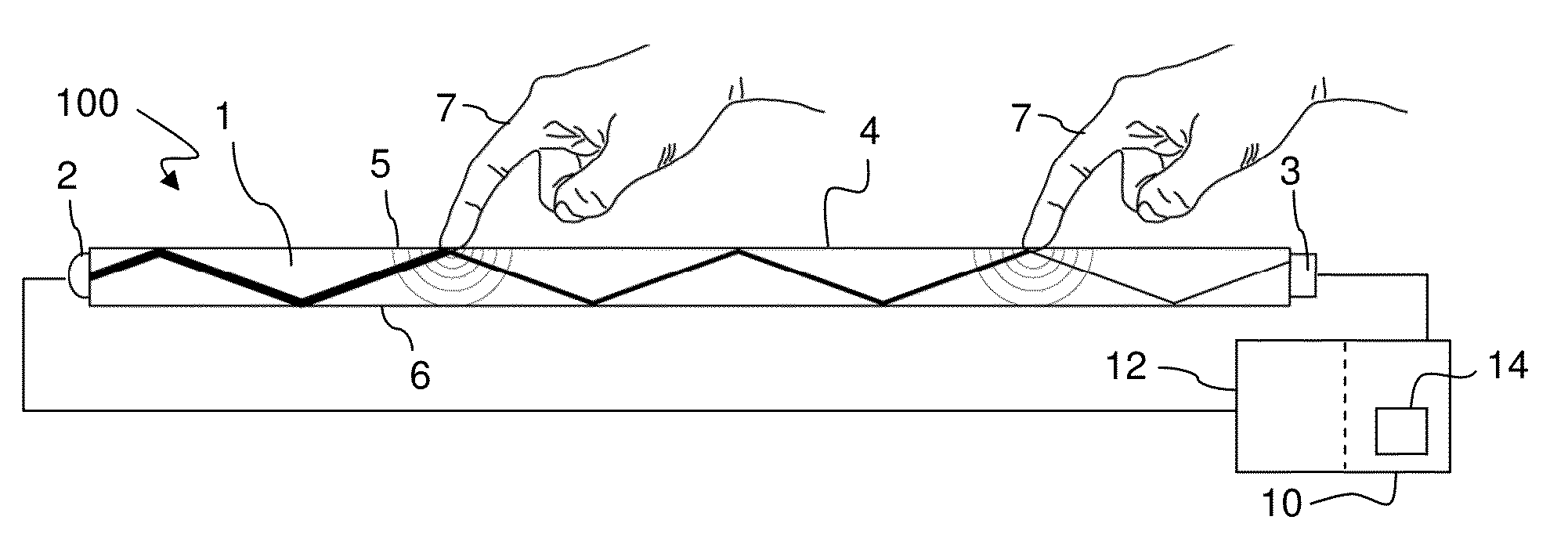
[0051]Embodiments of the inventions relate to signal processing in relation to a touch-sensitive apparatus which is based on the concept of transmitting energy of some form across a touch surface, such that an object that is brought into close vicinity of, or in contact with, the touch surface causes a local decrease in the transmitted energy. The apparatus may be configured to permit transmission of energy in one of many different forms. The emitted signals may thus be any radiation or wave energy that can travel in and across the touch surface including, without limitation, light waves in the visible or infrared or ultraviolet spectral regions, electrical energy,...
PUM
 Abstract
Description
Claims
Application Information
 - Generate Ideas
- Intellectual Property
- Life Sciences
- Materials
- Tech Scout
- Unparalleled Data Quality
- Higher Quality Content
- 60% Fewer Hallucinations
Browse by: Latest US Patents, China's latest patents, Technical Efficacy Thesaurus, Application Domain, Technology Topic, Popular Technical Reports.
© 2025 PatSnap. All rights reserved.Legal|Privacy policy|Modern Slavery Act Transparency Statement|Sitemap|About US| Contact US: help@patsnap.com