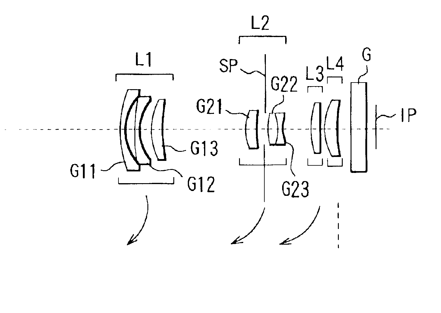
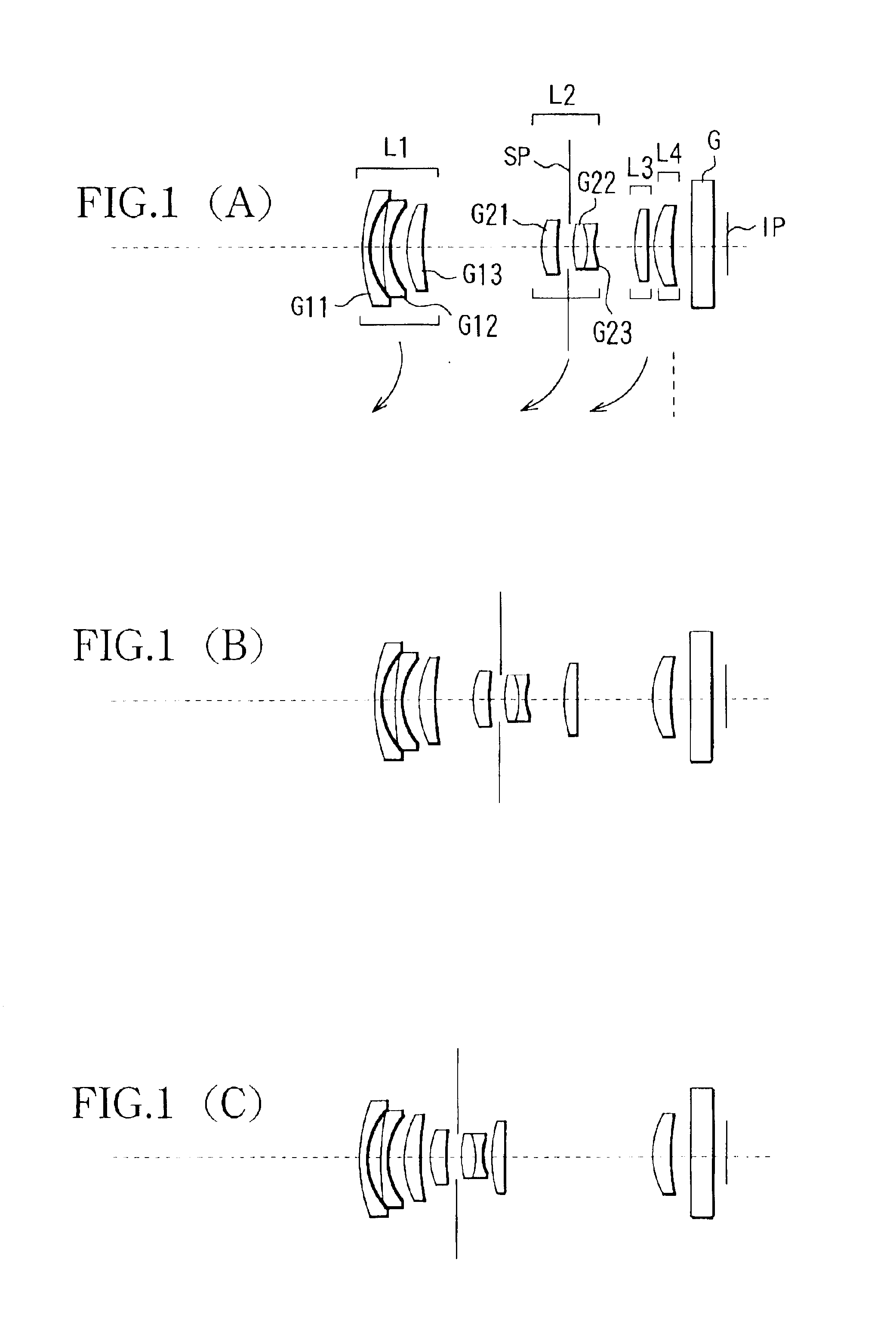
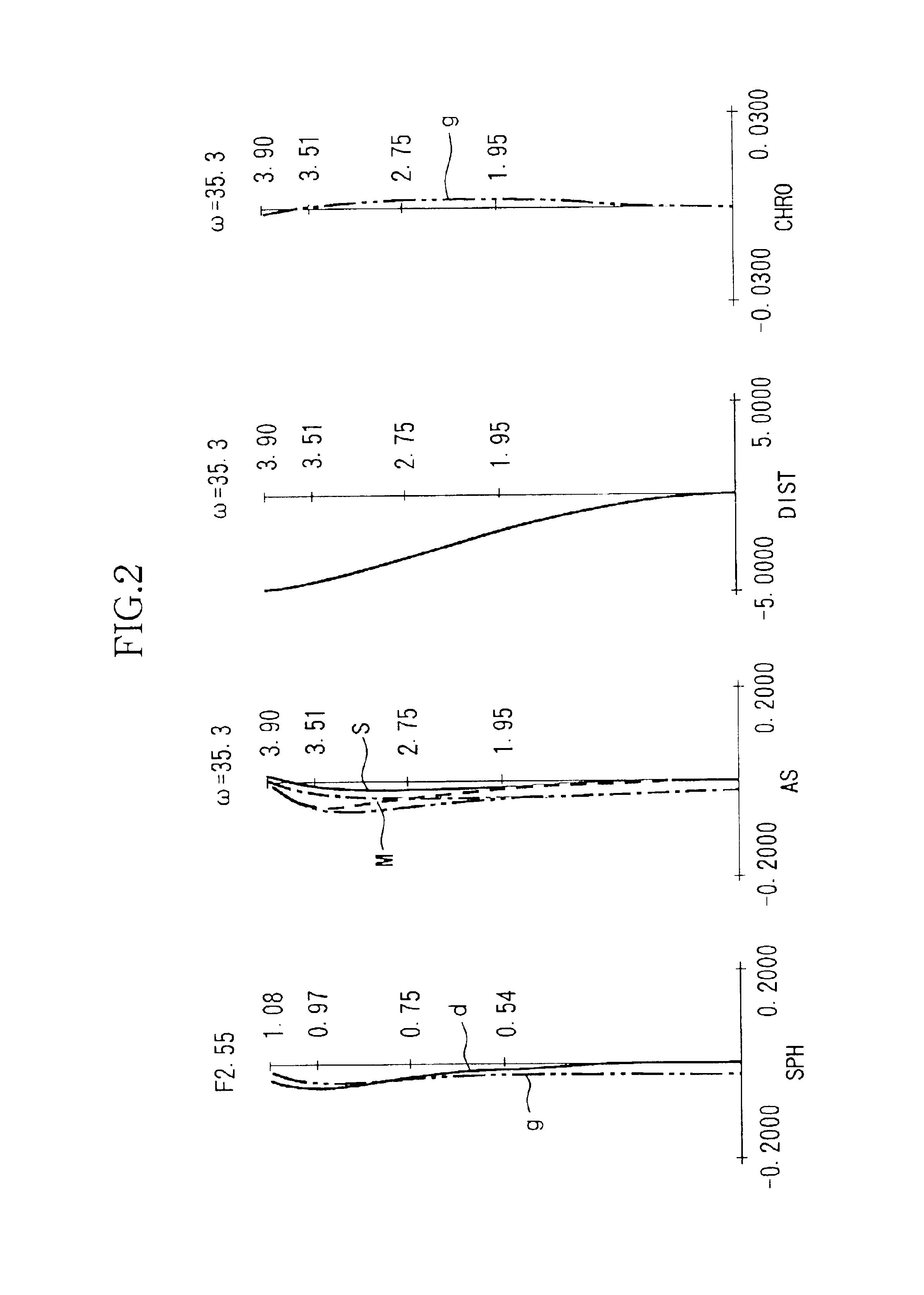
Zoom lens and camera

Abstract

The present invention discloses a zoom lens including:a first lens unit having negative optical power, the first lens unit having a negative lens element on a closest side to an object;a second lens unit having positive optical power, the second lens unit having two or more positive lens elements;a third lens unit having positive optical power; anda fourth lens unit having positive optical power, the fourth lens unit consisting of one positive lens component, said units arranged in the order presented from an object side to an image side,wherein at least the second lens unit and the third lens unit are moved toward the object for zooming from a wide angle side to a telephoto side such that a space between the first lens unit and the second lens unit is smaller, a space between the second lens unit and the third lens unit is smaller, and a space between the third lens unit and the fourth lens unit is larger at a telephoto end than at a wide angle end.Thus, a zoom lens having fewer lenses, a compact body, and good optical performance, and a camera using the same can be realized.

Description

BACKGROUND OF THE INVENTION[0006]1. Field of the Invention[0007]The present invention relates to a zoom lens suitable for a camera such as a digital still camera or a digital video camera, and more particularly to a portable zoom lens with reduced variation in exit pupil positions during zooming, an increased angle of view, and a reduced total length of lenses.[0008]2. Description of the Related Art[0009]Digital still cameras and digital video cameras using a solid-state image pickup device have recently become multifunctional, and optical systems used therein have needed both high optical performance and reduced size.[0010]Generally, a zoom lens used for a camera with a CCD such as a video camera is of a type including three to five lens units, a front lens unit among them consisting of lenses having positive, negative and positive refractive power, and a lens unit closest to an object being fixed during zooming.[0011]For example, Japanese Patent Laid-Open No. 63-81313 proposes a z...

AI Technical Summary

Benefits of technology

The present invention provides a zoom lens with fewer lenses, a compact body, and good optical performance. The lens has a negative front lens unit with a wide angle of view and high optical performance across the zoom range. The invention simplifies the total lens system by appropriately setting the refractive power of each lens unit or the material of a lens. A camera using the zoom lens is also provided.

Problems solved by technology

A zoom lens with large exit pupil variation of a lens system during zooming can be used as a zoom lens for a silver camera, but when used for an electronic still camera with a CCD, power distribution is limited from a design viewpoint to increase a size of the total lens system.

If the refractive power distribution of each lens unit, the lens configuration, and the material of the lens are inappropriately selected, aberration variation, particularly chromatic aberration variation in accordance with zooming increases to cause difficulty in achieving high optical performance across the zoom range.

Thus, if the first lens unit is to consist of two lenses: a negative lens and a positive lens, the negative lens requires an aspheric lens with a large deflection ratio between center thickness and edge thickness to cause difficulty in manufacturing.

Images