Ways to Optimize Resource Allocation

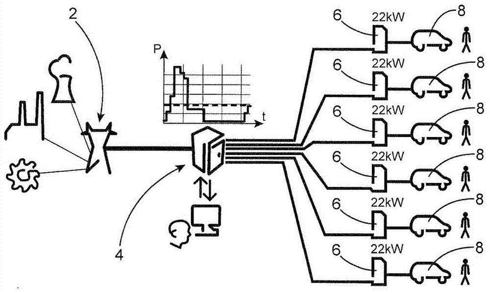
[0061] The following description is provided with reference to the drawings, figure 1 A system for providing electrical energy for electric and/or hybrid vehicles is shown in a schematic diagram. For example, the system includes an electrical energy source 2, which is connected to six charging terminals 6 through a management unit 4, each of which is Both have a rated power of 22kW. If the operator of the system wants to always charge the vehicle 8 with full power, he must obtain a contract of 6×22=132kW. Perhaps this maximum power is only occasionally reached. The required peak value represents an additional cost to the operator and may also be problematic for the power producer, who needs to invest in supplementary generating equipment to absorb temporary peaks. If the contract obtained is of a lower functional level, these peaks of demand will be sufficient to shut down the device and thus all charging terminals are unavailable.

[0062] Therefore, it is desirable to satisfy the charging requirements/requests of the vehicle 8 and the restriction conditions and goals of operation.

[0063] For this purpose, the solution according to the present invention is based on two phases, namely, a preliminary analysis phase and a subsequent phase of controlling the charging power.

[0064] The analysis phase includes notifying the charging requirements to the management unit 4, which considers the total energy available, cost constraints, and constraints specific to each vehicle to evaluate these requirements.

[0065] If the request is feasible and confirmed, the management unit 4 starts to allocate energy to the vehicle 8; otherwise, the management unit provides alternative solutions, such as allocating the requested energy but extending the charging duration, or maintaining the charging duration by allocating a smaller amount of energy time.

[0066] The stage of controlling the charging power includes: when a group of charging requests is received and the management unit 4 starts to satisfy these requests, calculating a resource allocation curve for each vehicle to be charged.

[0067] This calculation allows the main constraints (total available power, restrictions on each terminal and vehicle, time availability, etc.) and is adjusted in order to, for example, optimize a single objective selected from the following objectives: complete charging as quickly as possible, exhaust May start charging late, minimize costs, or carbon dioxide (CO 2 ) Footprint.

[0068] The distribution curve can be expressed as the magnitude of the intensity as a function of time, that is, the power (kW) as a function of time or the current intensity (A) as a function of time.

[0069] figure 2 Is in figure 1 A schematic diagram of the general structure of the charging management system in the application. The structure includes: a gateway layer 10 for application management, interpretation and communication purposes, providing interfaces with external participants (charging station operators, vehicle users, and vehicles); and a central core 12 for constructing resource allocation plans and Communication with the charging station operator 14 via the operator MMI15, with the user 16 of the vehicle 8 via the user MMI17, and with the vehicle 8 via the charging terminal 6 is performed.

[0070] A set of charging requests can be represented in the form of a Tasks object with the following parameters:

[0071] energyToAllocateKWh: the energy to be allocated [in kWh];

[0072] startTimeMin: The time at which charging can start [in minutes];

[0073] endTimeMin: The time at which charging cannot be performed since then [in minutes];

[0074] minCurrentA: The minimum current [in A] that must be allocated in order to charge the vehicle (charger activation threshold);

[0075] maxCurrentA: The maximum current intensity [in A] that can charge the vehicle (the limit value of the charging terminal, charging cable or vehicle charger).

[0076] It should be noted that each of these parameters is defined for each vehicle to be charged.

[0077] On the other hand, the available power and optimization data are expressed as follows:

[0078] availablePowerKW: The curve of the total available power [in kW] of the charging station as a function of time. At each moment, the sum of all the power allocated for each charge cannot be greater than the available curve;

[0079] energeticalCostEur: Energy cost [in Euros per kilowatt hour (EUR/kWh)] as a function of time;

[0080] CO2Emissions: the equivalent CO generated by electricity 2 Curve of emissions [in gCO2eq/kWh] as a function of time.

[0081] In the following, the indicators for each of these variables are used as follows: "i" indicates the terminal that charges a given vehicle; and "j" indicates the time period considered according to the discretization of the time performed.

[0082] The variable name and unit selection given here are examples.

[0083] Based on this definition, the solution to the problem includes:

[0084] -Evaluate its feasibility; this stage includes verifying whether it is possible to define a set of resource allocation curves that allow the requested energy to be allocated to obey the defined constraints (constraints on the curve, constraints on the available resources, and time constraints).

[0085] -Define the optimal allocation curve allocationCurrentA (allocated current [in A], for each terminal i connected to the vehicle to be charged, and for each time period j).

[0086] image 3 Shown in figure 1 In the case of the exemplary embodiment, the main steps of the method according to the present invention.

[0087] In the analysis phase, the management unit 4 receives (step 20) problem data, in other words, the defined optimization goals (end charging as early as possible, start charging as late as possible, minimizing costs and minimizing carbon traces), The constraints, the total available energy, and the cost of meeting these goals.

[0088] In step 22, define the time domain of the problem, in other words, the total time interval available for charging the vehicle 8, and divide the duration into equal time periods corresponding to a single time slot with the same constraint conditions . Therefore, the division is performed in such a manner that the number of time periods to be processed is limited to the number that is definitely necessary. In the exemplary embodiment described here, each section (section) is defined by the start time, duration, available power, price per kWh consumed, and the number (indicator) of the terminal that can be requested.

[0089] In step 24, priority rules are defined between different charging requesters.

[0090] In step 26, the processing sequence of the defined time period is defined for each charging requester, and in step 28, a charging curve is constructed for each request. in Image 6 This step is described in detail.

[0091] In step 30, the management unit 4 makes a determination as to whether optimized charging is feasible or not.

[0092] Figure 4 Is a schematic diagram of an example of the change in energy cost as a function of time in a given time period.

[0093] In this example, consider the following conditions:

[0094] Time range=[30,240] (in minutes)

[0095] Charge request at terminal 1, availability interval [30,240]

[0096] Charge request at terminal 2, availability interval [60,180]

[0097] Constant available power during H;

[0098] Energy cost: through Figure 4 The curve is given.

[0099] Discretization in the time domain leads to Figure 5 , Of which, 5 time periods ① to ⑤ are limited.

[0100] according to image 3 Step 24 of the flowchart is to establish a priority order for processing charging requests of different vehicles. The processing order of this type can be limited to multiple levels. When leaving this step, a vector called taskPriorityOrder is obtained by indexing requests sorted in priority order. As an illustration, consider the following example:

[0101] Request at terminal 1:

[0102] Priority=1

[0103] startTimeMin=10

[0104] endTimeMin=180

[0105] Request at terminal 2:

[0106] Priority=1

[0107] startTimeMin=20

[0108] endTimeMin=100

[0109] Request at terminal 3:

[0110] Priority=2

[0111] startTimeMin=15

[0112] endTimeMin=120

[0113] Request at terminal 4:

[0114] Priority=2

[0115] startTimeMin=10

[0116] endTimeMin=120

[0117] The priority rules are defined as follows:

[0118] The first classification level: priority levels in increasing order (requests with low priority levels are preferred)

[0119] The second classification level: endTimeMin in increasing order (requests to be terminated faster have priority)

[0120] The third classification level: startTimeMin in increasing order (requests that can start later have priority)

[0121] These classification rules return the vector taskPriorityOrder=[2;1;3;4].

[0122] Then, for each charging request, you can use image 3 Step 26 of the flowchart defines the processing sequence for the relevant time period. This sequence can be used to adjust the selected optimization as follows:

[0123] For example, if it is desired that resource allocation ends as early as possible, the time period is processed by starting from the earliest one time period and proceeding in chronological order.

[0124] If it is desired to provide "just in time" resource allocation (where each allocation is completed as late as possible), it is processed by starting from a time period completed as late as possible and proceeding in reverse chronological order period.

[0125] If the energy cost is to be minimized, the processing priority is given to the time period with the lowest energy cost: therefore, the processing order is obtained by dividing the time period in the order of increasing energy cost.

[0126] If carbon traces are to be minimized, priority is given to equal CO with generated electrical energy 2 Time period of the lowest indicator of emission: Therefore, the processing order is obtained by dividing the time period in the ascending order of the indicator.

[0127] Other optimizations can be provided by assigning specific coefficients to each time period and by performing incremental or decremental classification on these coefficients. This method makes it possible to achieve global optimization goals (using the same rules for all requests) or to provide specific optimizations for each request.

[0128] At the end of this step, a timeSectionFillingOrder matrix is ​​obtained, where each column corresponds to the request, and the index of the time period to be processed according to the defined order is entered in the row.

[0129] Therefore, with these constraints, in the case of a request at the terminal 1, if the resource allocation is required to end as late as possible, the following vector is obtained:

[0130] timeSectionFillingOrder(:,1)=[1;2;3;4;5]

[0131] If you want to provide "just in time" resource allocation, you get the following vector:

[0132] timeSectionFillingOrder(:,1)=[5;4;3;2;1]

[0133] If the energy cost is to be minimized, the following vector is obtained:

[0134] timeSectionFillingOrder(:,1)=[3;4;1;2;5],

[0135] For time periods with the same energy cost, classification by increasing time period indicators is performed.

[0136] Image 6 The specific details of the operation of step 26 for constructing the resource allocation curve are shown.

[0137] In step 40, after the request is processed at a given time, the next request is considered in the vector taskPriorityOrder, and then the next time period is considered in the vector timeSectionFillingOrder, and by reference Figure 7 Describe the process in detail to allocate resources.

[0138] In step 46, it is checked whether the allocated energy is greater than the requested energy.

[0139] If the allocated energy is less than the requested energy, it is checked (step 48) whether the time period being processed is the last time period. If the time period is not the last time period, the process continues from step 42. However, if the time period is the last time period, it is checked (step 50) whether the request being processed is the last request.

[0140] If the request being processed is not the last request, the procedure continues from step 40.

[0141] If the request being processed is the last request, the management unit 4 generates an allocation curve allocationCurrent A for each request.

[0142] If in step 46, the allocated energy is found to be greater than or equal to the requested energy, the procedure starts from step 50.

[0143] In step 54, the management unit 4 checks whether the allocated energy is greater than or equal to the requested energy.

[0144] If the allocated energy is greater than or equal to the requested energy, the management unit generates (step 56) a positive determination of the feasibility of optimized charging according to the defined allocation curve.

[0145] If not, the management unit 4 generates (step 58) a negative judgment on the feasibility of optimizing charging according to the defined distribution curve.

[0146] Figure 7 Shows the distribution of energy used in each time period Image 6 The specific details of the operation of the steps.

[0147] The requests are processed one by one in the order defined in taskPriorityOrder. For each request, according to the order defined in timeSectionFillingOrder, resource allocation is performed on each time period until the requested energy is fully allocated.

[0148] Figure 7 The flowchart includes 3 main functional areas.

[0149] There is area A where the process considers resource requests that can be made through charging tasks that have not yet been processed. Here, the purpose is to try to keep resources in reserve for these future requests if possible. If it is found that the available resources are insufficient to satisfy the (minimum) future request, all available resources are allocated to the task being processed.

[0150] There is a region B, in which, for the task being processed, the distribution current is limited according to the constraint condition maxCurrentA.

[0151] There is a region C where, when the current is distributed during the time period being processed, it is checked whether the total energy allocated to the task is greater than the energy originally requested. If so, keep the current distribution value and reduce the time period to a time period that is really necessary.

[0152] It should be noted that an alternative method of dealing with this situation can be to keep the time period unchanged, and reduce the distributed current to a current that is indeed necessary.

[0153] Therefore, in step 60, for a given time period j, the management unit 4 calculates the available current availableCurrentA_j in the time period.

[0154] In step 62, the available current availableCurrentA_j is compared with minCurrentA_i, where minCurrentA_i represents the minimum current that must be allocated in order to allow the vehicle to charge at the terminal i. This value corresponds to the charger trigger threshold.

[0155] If availableCurrentA_j is greater than minCurrentA_i, perform the steps of area A.

[0156] If availableCurrentA_j is less than minCurrentA_i, the allocation current allocationCurrentA_ij takes a zero value (step 90) and the allocation process of terminal i in time period j is terminated.

[0157] In area A, in step 64, the management unit 4 checks whether the resources are sufficient for allocating the lowest minimum current that can be requested by another charging task.

[0158] If the resources are not enough to allocate the lowest minimum current requested through another charging task, then in step 65, the available current availableCurrentA_j is completely allocated through the terminal i.

[0159] If the resources are sufficient to allocate the minimum minimum current requested by another charging task, then in step 66, the management unit 4 checks whether the resources are sufficient to allocate the minimum current to all requests within the time period j.

[0160] If the resources are insufficient to allocate the minimum current to all requests, in step 67, the management unit 4 allocates the current minCurrentA_i through the terminal i.

[0161] If the resources are sufficient to allocate the minimum current to all requests, the management unit 4 calculates compAllocationA_ij, which represents the supplementary current that can be allocated after subtracting all the minimum currents in the fair sharing configuration, and allocates (step 70) the current minCurrentA_i+compAllocationA_ij.

[0162] The resource allocation process continues from the steps of area B and area C.

[0163] In step 80, the allocated current allocationCurrentA_ij is compared with maxCurrentA_i, where maxCurrentA_i represents the maximum value that the vehicle can be charged through the terminal: for example, the value may be the limit value of the charging terminal i, the charging cable, or the vehicle charger.

[0164] If allocationCurrentA_ij is greater than maxCurrentA_i, the allocated current is limited to maxCurrentA_i (step 82).

[0165] If allocationCurrentA_ij is less than or equal to maxCurrentA_i, the method continues through the steps of area C.

[0166] In step 84, the allocated energy is compared with the requested energy.

[0167] If the allocated energy is greater than the requested energy, the calculated allocated current value is retained (step 86), but the time period is reduced to a time period that is indeed necessary. This requires dividing the time period into two parts and a new discretization of the time domain. So far, the allocation process of terminal i ends.

[0168] If the allocated energy is less than or equal to the available energy, the resource allocation of the terminal i in the time period j is terminated.

[0169] will be Figure 8 to Figure 11 Illustrated in the exemplary application shown Image 6 with Figure 7 Describe the process.

[0170] Consider the following requests at terminals 1 and 2:

[0171] Terminal 1:

[0172] energyToAllocateKWh_1:14.4kWh

[0173] startTimeMin_1:30min

[0174] endTimeMin_1:240min

[0175] minCurrentA_1:6A

[0176] maxCurrentA_1:32A

[0177] Terminal 2:

[0178] energyToAllocateKWh_1: 4.32kWh

[0179] startTimeMin_1:60min

[0180] endTimeMin_1:180min

[0181] minCurrentA_1:6A

[0182] maxCurrentA_1:32A

[0183] It is charged in three-phase mode and the phase neutral point voltage on the entire charging station is constant PNVoltage=240V.

[0184] The available power of the charging station is constant in all the time domains discussed, at availablePowerKW=8.64kW (corresponding to a current of 12A).

[0185] Assume that the previous example ( Figure 4 ) The energy cost is the same as the energy cost.

[0186] Therefore, the same time discretization as before is used.

[0187] Figure 8 The result of this time discretization is shown.

[0188] For the task processing sequence, the following rules apply:

[0189] The first classification level: the end time endTimeMin in increasing order (requests that terminate sooner take precedence)

[0190] The second classification level: the start time startTimeMin in increasing order (requests that can start later are preferred)

[0191] Classification level 3: No level 3 exists

[0192] Therefore, we get the task priority order taskPriorityOrder=[2;1]

[0193] The strategy to be used is to minimize energy costs. Therefore, we obtain the following sequence of processing time periods:

[0194] Request 1: Time Section Filling Order timeSectionFillingOrder(:,1)=[3;4;1;2;5]

[0195] Request 2: Time Section Filling Order timeSectionFillingOrder(:,2)=[3;2]

[0196] Therefore, subject to the following constraints, use Image 6 Curve construction flowchart.

[0197] The first task to be processed is number 2 and we start from time period 3: we start from Figure 7 The allocation process shown begins.

[0198] -The allocation has not been performed so far; therefore, the available current availableCurrentA_3=12A.

[0199] -The available current is greater than minCurrentA_2=6A, therefore, we enter area A. The only other request that can be processed in time period 3 is request 1, for which minCurrentA_1=6A. Therefore, the available current is sufficient to provide the minimum allocation for all tasks in this time period; however, after the allocation, there are no more available resources in this time period. Therefore, we calculate the supplemental allocation compAllocationA_23=0A to obtain:

[0200] allocationCurrentA_2,3=minCurrentA_2+compAllocationA_2,3=6A

[0201] -AllocationCurrentA_2,3 is less than the maximum current maxCurrentA_2, so we move to area B without modification.

[0202] -Then, we enter area C. The duration of time period 3 is 90 minutes. Therefore, the energy allocated by the current allocationCurrentA_2,3=6A in the entire cycle is:

[0203] 6A*240V*3*90min=388,800W min=6.48kWh

[0204] This energy is greater than the requested amount, which is 4.32 kWh. Therefore, reduce the time period to a time period that is really necessary, in other words, a duration of 60 minutes (6A*240V*3*60min=259,200W min=4.32kWh). Insert a new time period starting from 150 minutes and having a duration of 30 minutes.

[0205] Then, the distribution curve has Picture 9 The level shown.

[0206] The second task to be processed is number 1, and we start from time period 3. This time period is only divided into two parts: the first part that starts from 90 minutes and has a duration of 60 minutes as indicated by indicator 3a; and the first part that starts from 150 minutes and has a duration of 30 minutes as indicated by indicator 3b the second part.

[0207] In time period 3a, Figure 7 The distribution process shown is applied to terminal 1. At the end of this step, the allocated energy is less than the requested energy, and there is still some time period that is not completed for request 1. according to Image 6 Steps 46 and 48, the allocation process continues in the time period 3b.

[0208] At the end of this step, the total energy allocation for request 1 has not yet been completed. in Picture 10 The distribution curve at this intermediate point is shown in.

[0209] We will continue to implement in the remaining time period to be considered for request 1. Image 6 with Figure 7 The process shown.

[0210] in Picture 11 The final distribution curve is shown in.