

Method for reconstructing curved surface of complex space
A technology of surface reconstruction and space, applied in image data processing, 3D modeling, instruments, etc., can solve problems such as surface reconstruction of complex geological structures, and achieve the effect of ensuring fast processing and ensuring accuracy
- Summary
- Abstract
- Description
- Claims
- Application Information
AI Technical Summary
Problems solved by technology
Method used
Image

Examples
Embodiment Construction
[0064] First define some basic geological structures and terms used in this plan:
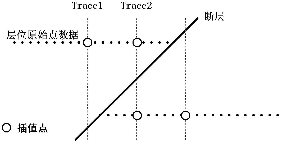
[0065] Horizon: It refers to a specific position in the stratigraphic sequence. The stratigraphic horizon can be the boundary of a stratigraphic unit, or it can be a marker layer belonging to a specific era, etc.
[0066] Fault: The crustal rock layer ruptures due to the force reaching a certain strength, and the structure that moves obviously relative to the rupture surface is called a fault.
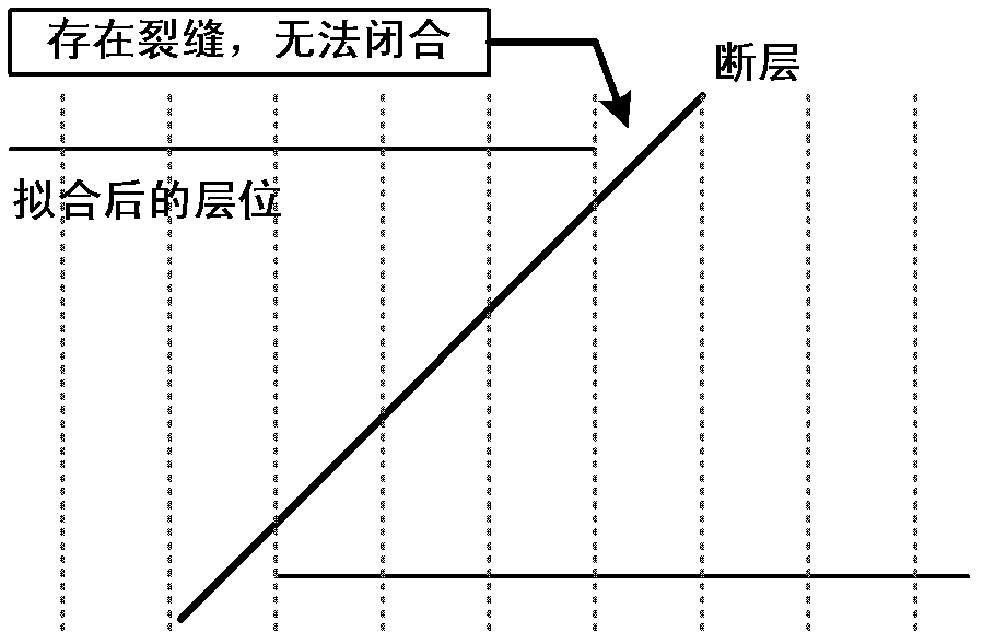
[0067] Vertical fault: A fault with a small fault throw.
[0068] Gridding: Logically divide the discrete point data to form a regular logical grid, which is convenient for horizon interpolation.
[0069] Interpolation: The process of using known points to calculate unknown points.
[0070] Fitting: A process of using the data after horizon interpolation to form horizons.
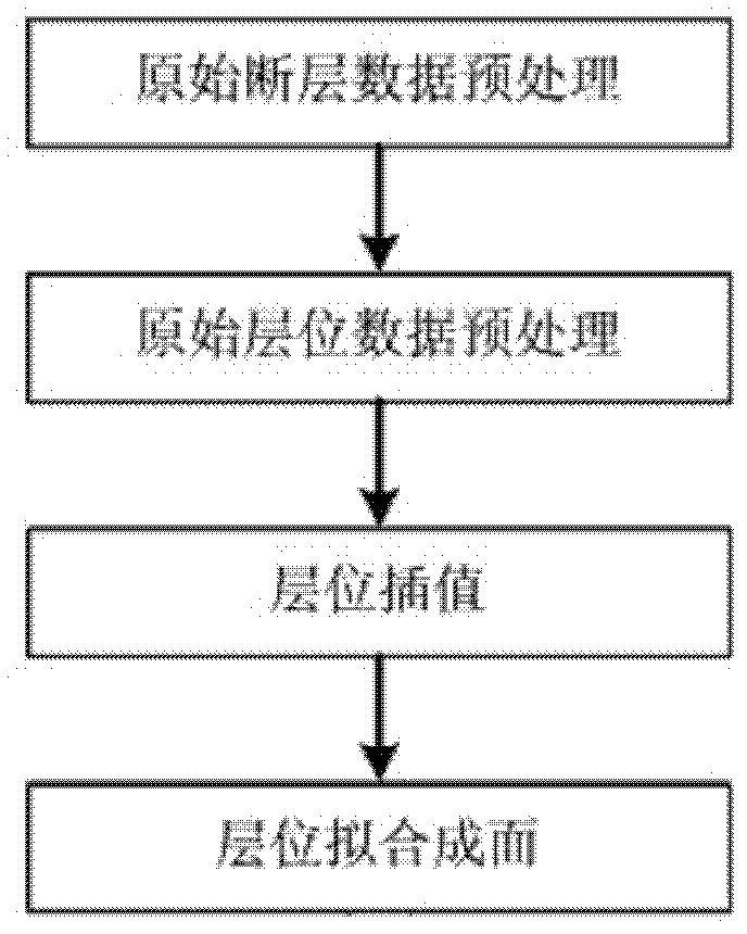
[0071] Such as image 3 As shown, a complex space surface reconstruction method includes the following steps:
[0...
PUM
 Abstract
Description
Claims
Application Information