

Failure recognition method and system based on neural network self-learning
A neural network and fault identification technology, which is applied in the direction of biological neural network models, can solve problems such as low efficiency, high risk, and heavy workload, and achieve faster speed, faster fault identification, and labor cost savings.
- Summary
- Abstract
- Description
- Claims
- Application Information
AI Technical Summary
Problems solved by technology
Method used
Image

Examples
Embodiment Construction
[0037] The present invention will be described in detail below through specific embodiments and accompanying drawings.
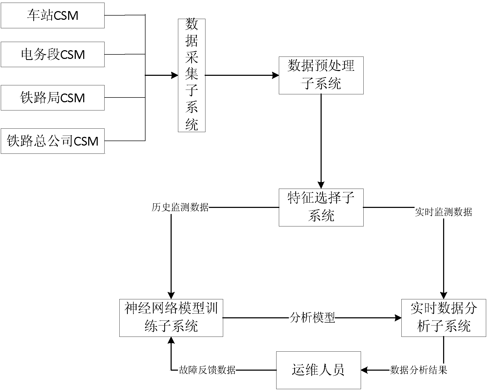
[0038] A fault identification method and system based on neural network self-learning in this embodiment is composed of the following parts: CSM-based data acquisition subsystem, data preprocessing subsystem, feature selection subsystem, model training subsystem, real-time data analysis subsystem system and self-learning subsystem. It is used to solve technical problems such as large workload, low efficiency and high risk in manual diagnosis of railway signal system faults in the prior art.
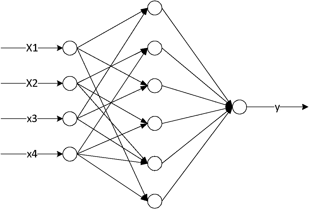
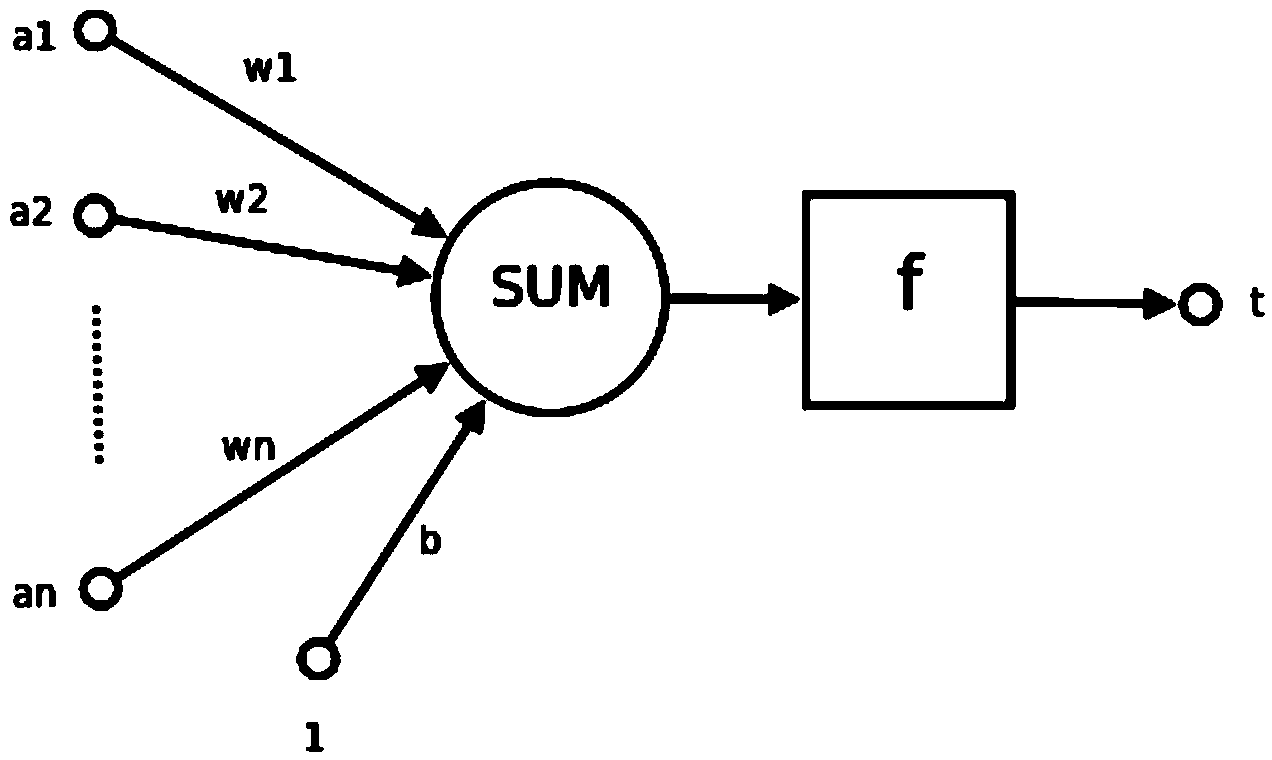
[0039] The neural network is mainly composed of neurons, and the structure of neurons is as follows: figure 2 As shown, a1~an are the components of the input vector
[0040] w1~wn are the weights of each synapse of neurons
[0041] b is bias
[0042] f is a transfer function, usually a nonlinear function. Generally, there are sigmod(), traind(), tansig(), hardlim()....
PUM
 Abstract
Description
Claims
Application Information