

EOF-based unmanned aerial vehicle signal identification system and method
A signal recognition and UAV technology, applied in the field of UAV identification, can solve the problem of difficult identification of similar UAV signals, achieve good support, improve the recognition effect, and improve the effect of the recognition effect.
- Summary
- Abstract
- Description
- Claims
- Application Information
AI Technical Summary
Problems solved by technology
Method used
Image

Examples
Embodiment Construction
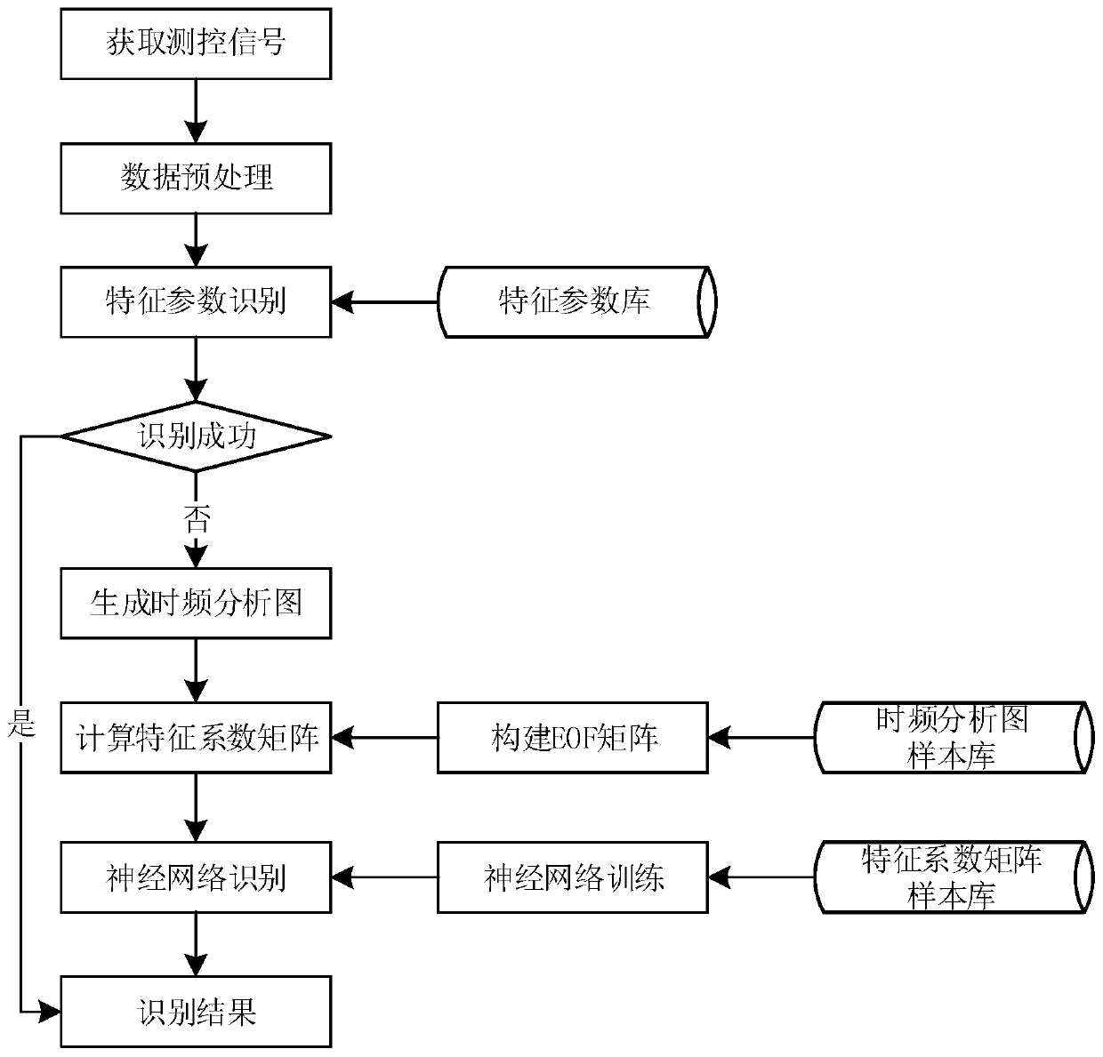
[0043] Embodiments of the present invention will be described in further detail below in conjunction with the accompanying drawings.
[0044] Aiming at the problem that similar UAV signals are difficult to recognize, the invention proposes an EOF-based UAV signal recognition method. The specific principle of EOF is described below.
[0045] Empirical Orthogonal Function (EOF) is an analysis method that separates the contributions of different physical processes and mechanisms to variable fields through the analysis of observed data. The basic idea of the EOF method is that a large amount of related data must always have a common factor that dominates it. Under the condition of not losing or losing as little information as possible in the original data, the original data is simplified to extract the characteristic information of the original data. Using the EOF method, we can identify the main mutually orthogonal spatial distribution patterns from the data set of the variabl...
PUM
 Abstract
Description
Claims
Application Information