Bit-rate guided frequency weighting matrix selection

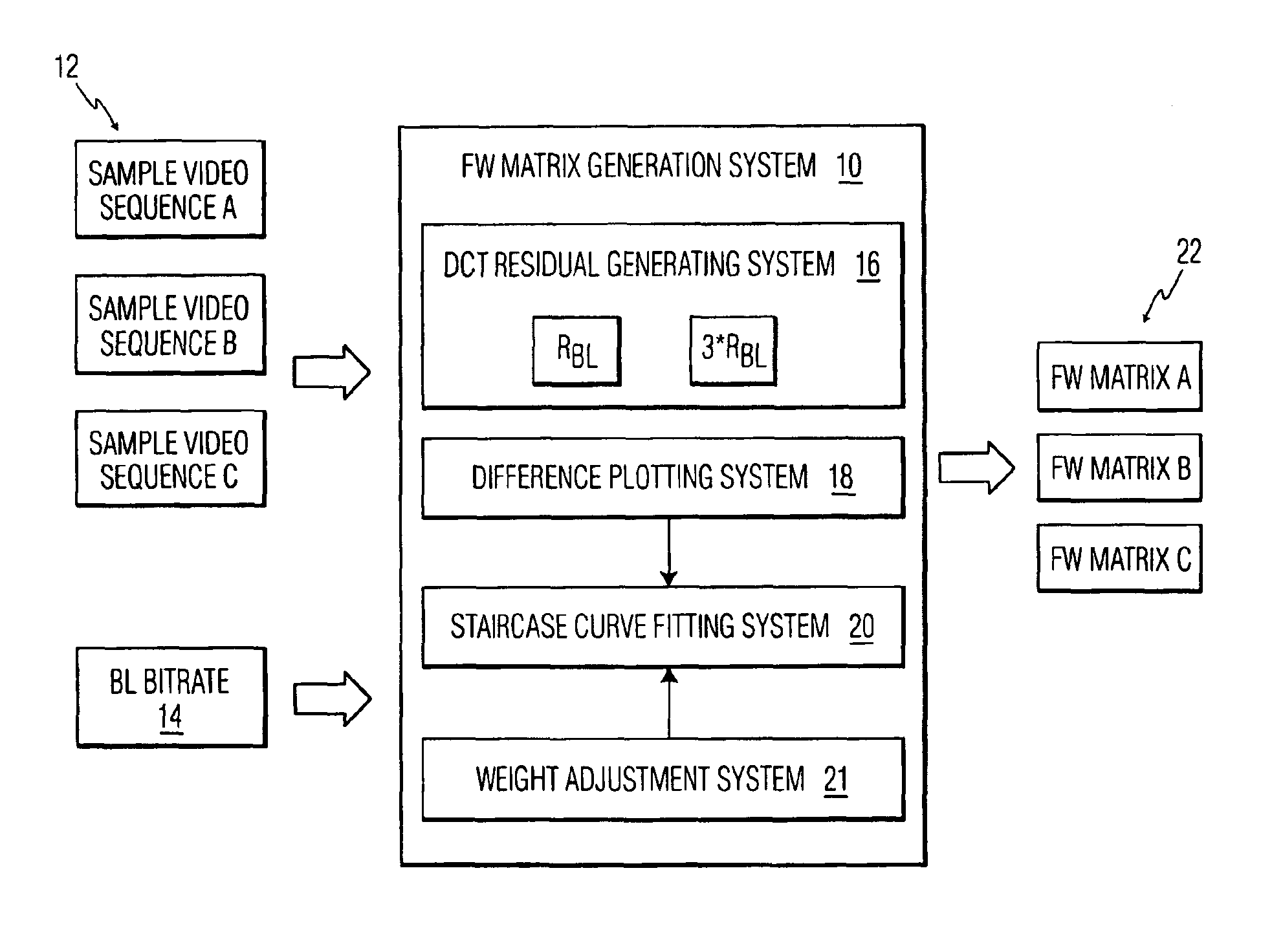
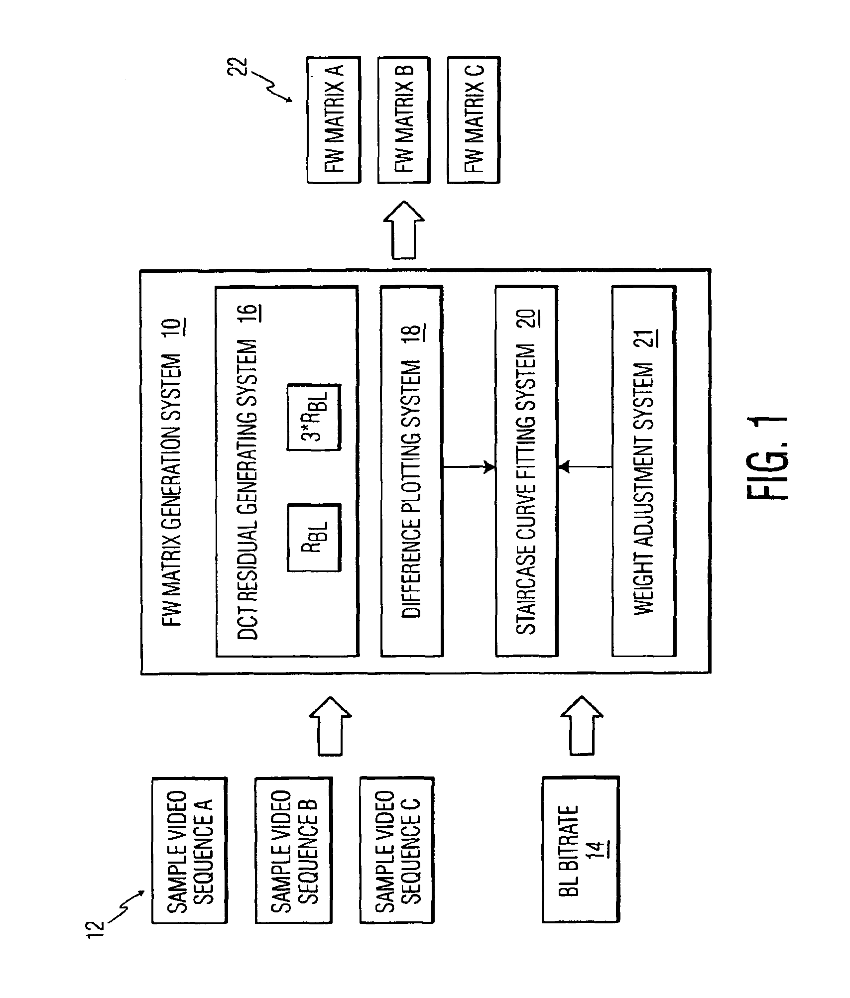
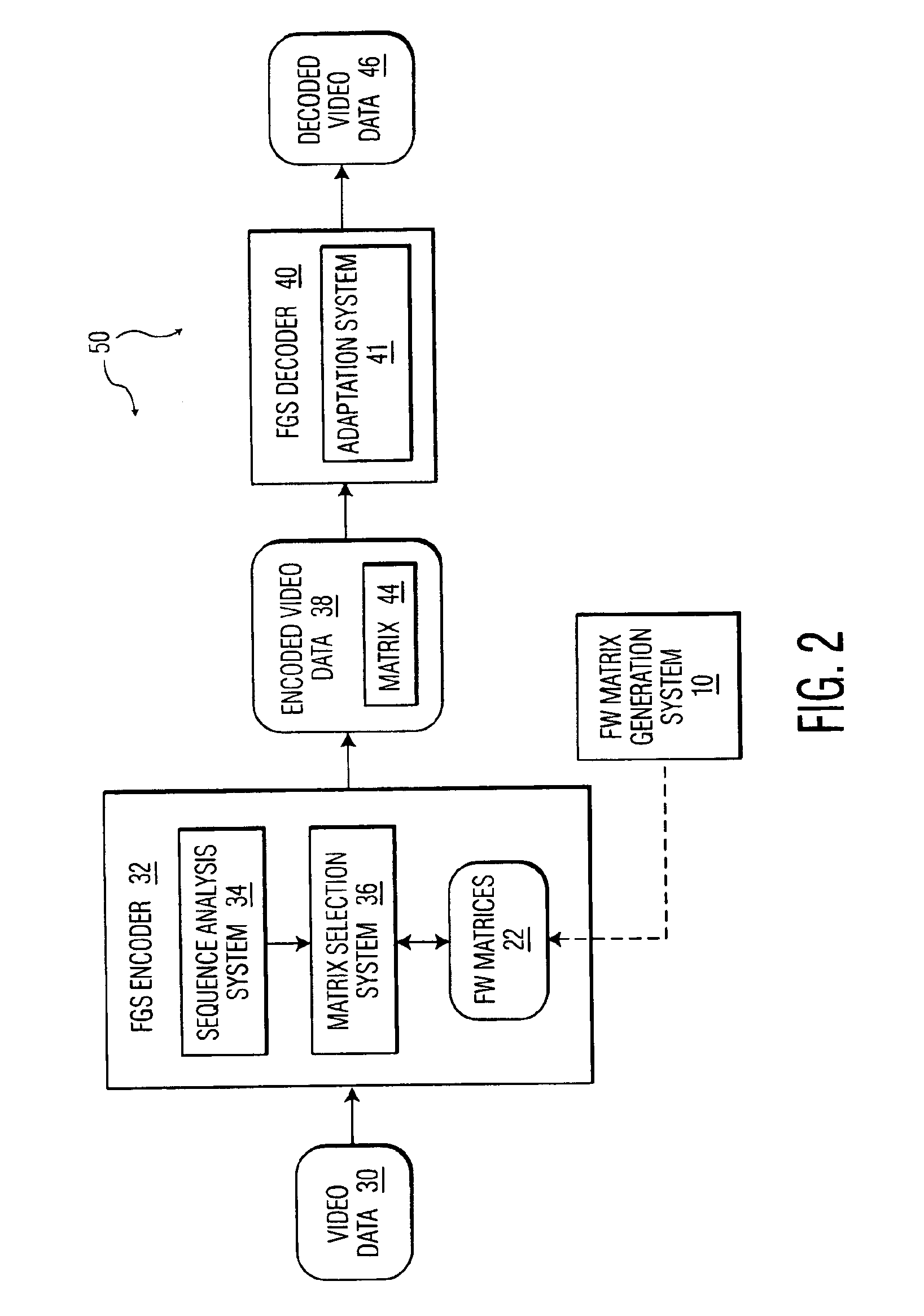
[0023]Referring now to the drawings, FIG. 1 depicts a Frequency Weighting (FW) Matrix Generation System 10 that receives one or more sample video sequences 12 and a base layer (BL) bit-rate 14, and outputs a set of FW matrices 22. Each sample video sequence 12 includes a unique scene type or characteristic that might typically be processed by a Fine-Granularity-Scalability (FGS) system, such as that sown in FIG. 2. Thus, for example, “Sample Video Sequence A” might comprise a high activity scene, “Sample Video Sequence B” might comprise a medium activity scene, and “Sample Video Sequence C” might comprise a low activity scene.

[0024]FW Matrix Generation System 10 generates a unique FW matrix for each inputted sample video sequence, so that each FW matrix is associated with a predetermined scene type. Thus, for instance, FW matrix A would correspond to a high activity scene, FW matrix B would correspond to a medium activity scene, and FW matrix C would correspond to a low activity. The number of FW matrices 22 generated can vary depending on the anticipated FGS application. Simple applications, such as a videophone, may require only single matrix derived from a low activity, low motion sample video sequence. Other more complicated applications may require a database of matrices to handle many different scene types. Moreover, any criteria (e.g., activity, motion, brightness, etc.) within a scene can be used to distinguish one sample video sequence (and therefore FW matrix) from another.

[0025]In the embodiment of FIG. 1, FW matrix generation system 10 utilizes a DCT residual generating system 16, a residual difference plotting system 18, a staircase curve fitting system 20, and a weight adjustment system 21 to generate FW matrices 22. The operations of these systems are described in further detail below.

[0026]FW matrix generation system 10 determines weights for each matrix from a staircase curve match of the difference of the average discrete cosine transform (DCT) residuals of a sample video frame calculated at critical bit-rates that generally include: (1) a selected bit-rate, and (2) a multiple of the selected bit-rate. The critical bit-rates can be selected as any value depending on, e.g., the particular application, resolution/size, frame rate, etc.

[0027]In an exemplary embodiment, the critical bit-rates comprise the base layer coding bit-rate (RBL) 14, and three times the base layer coding bit-rate (i.e., 3*RBL). Various experiments have shown that the largest quality gap between SLS and FGS appears at approximately three times the FGS BL bit-rate. For instance, the following analysis on a “Foreman” sequence shows that the RBL and 3*RBL are critical bit-rates. FIG. 4 shows the peak signal-to-noise ratio (PSNR) of a “Foreman” video sequence encoded with a non-scalable coder (i.e., SLS-single layer switching) and with an FGS encoder having a base layer bit-rate of 100 kbps. As can be seen, in the 100 kbps-1 Mbps bit-rate range, the largest PSNR quality penalty gap between FGS and a non-scalable coder is around 300 kbps. Thus, FGS and SLS has a critical quality gap at 3*RBL. Hence, in this embodiment, the FW matrix selection is based on the average DCT residual values at critical quality bit-rates 3*RBL and RBL, and the FW matrix selected using DCT residuals at these bit-rates should have a higher impact than ones selected at other bit-rates. It should be understood that other critical quality bit-rates and/or multiples of RBL (e.g., 2.5, 3.5, 4, 4.5, etc.) could be utilized to define the critical quality gap without departing from the scope of the invention.

[0028]FIG. 5 shows a 3-D mesh of frame-based difference of the average residual of the “Foreman” sequence at bit-rates of 100 kbps and 300 kbps. In this case, there are two scene types for the “Foreman” sequence. It is clear that for a particular scene characteristic, the residual characteristics are similar for all frames within the scene. Hence, a single frame from a sample video sequence can be utilized to generate the FW matrix for all the frames that have the similar scene characteristics.

[0029]Referring back to FIG. 1, the operation of FW matrix generation system 10 is described as follows. DCT residual generating system 16 generates (and plots) the average DCT residuals for a selected frame of the inputted video sequence at the critical quality bit-rates, in this case, RBL and 3*RBL. The average DCT residuals for each are plotted as a function of their location in a block of DCT data. Preferably, the residuals are extracted in a zigzag line from top left to bottom right (i.e., “DCT zigzag scan line”) to follow the energy dissipation trend. In the example shown here, coefficient numbers 1-64 provide the zigzag location for each residual inside an 8×8 DCT block. 1 2 6 7 | 15 16 28 29 3 5 8 14 | 17 27 30 43 4 9 13 18 | 26 31 42 44 10 12 19 25 | 32 41 45 54 - - - - + - - - - 11 20 24 33 | 40 46 53 55 21 23 34 39 | 47 52 56 61 22 35 38 48 | 51 57 60 62 36 37 49 50 | 58 59 63 64

[0030]The 64 residual values would then be plotted as shown in FIG. 6. FIG. 6 shows an exemplary plot of the 50th frame of the “Foreman” sequence of FIG. 5 at SLS coding bit-rates of 100 kbps and 300 kbps coded with an MPEG-4 non-scalable coder. From FIG. 6, it can be seen that the profiles of the DCT coefficient residuals at the two bit-rates are especially different for the lower frequency residuals. If the residual of the SLS at 100 kbps is coded in FGS enhancement layer, comparing the FGS and SLS at 300 kbps, it is clear that the quality gap between the FGS and the SLS coding are caused by the bit-plane cut-off of the FGS residuals at the transmission side. However, if the low frequency residuals get higher priority in the bit-plane coding through FW, the same bit-plane cut-off at the transmission side will result in smaller loss of the low frequency residuals at the receiver side, which in turn will bring better output quality for the FGS layer. The FW amount is dominated by the residual difference between these two bit-rates. The more the lower frequency residuals get compensated, the smaller the quality gap between the FGS and SLS at 300 kbps.

[0031]Next, difference plotting system 18 (FIG. 1) plots the difference of the average residual of the two DCT residual plots. FIG. 7 depicts an exemplary plot that shows the difference curve 60 of the average residuals for the two plots of FIG. 6 (i.e., the plot at 100 kbps minus the plot at 300 kbps). The difference curve 60 is plotted by DCT coefficient locations corresponding to a DCT zigzag scan line, as shown above. Staircase curve fitting system 20 then matches a staircase curve 62 to the difference curve 60.

[0032]Using the residual difference of the average DCT residuals based on two different bit-rates (e.g. 100 kbps and 300 kbps bit-rate) as a guideline, the FW matrix weights are selected using the staircase curve 62 matched to the shape of the residual difference. The matched staircase values for each DCT coefficient are then mapped into a FW matrix in the same zigzag configuration as described above. For example, in a four quadrant matrix made up of 64 elements arranged in a zigzag line from top left to bottom right to follow the energy dissipation, the DCT coefficient weights from the staircase curve would be arranged in the FW matrix as follows: 1 2 6 7 | 15 16 28 29 3 5 8 14 | 17 27 30 43 4 9 13 18 | 26 31 42 44 10 12 19 25 | 32 41 45 54 - - - - + - - - - 11 20 24 33 | 40 46 53 55 21 23 34 39 | 47 52 56 61 22 35 38 48 | 51 57 60 62 36 37 49 50 | 58 59 63 64

[0033]An exemplary FW matrix containing actual coefficient values would looks as follows: [ ⁢ 4 4 3 3 2 1 1 0 4 3 3 2 1 1 0 0 3 3 2 1 1 0 0 0 3 2 1 1 0 0 0 0 2 1 1 0 0 0 0 0 1 1 0 0 0 0 0 0 1 0 0 0 0 0 0 0 0 0 0 0 0 0 0 0 ⁢ ]

[0034]It is noted that the total number of bit-planes adopted in the system implementation may limit the weights of the FW matrix. In particular, when one or more of the weights selected by the staircase match are larger than the upper limit of the total number of bit-planes, the weights must be normalized by weight adjustment system 21. For instance, in FIG. 6, the first DCT coefficient has a weight of seven. However, if the number of bit-planes were limited to six, the weight of the first coefficient would exceed the upper limit. In this case, weight adjustment system 21 would modify the generated staircase curve by essentially shifting it to the left until the weight of the first coefficient equaled the upper limit of the total number of available bit-planes. In this manner, the normalized staircase curve is kept in parallel with the original staircase curve. It is understood that other adjustment algorithms could likewise be used without departing from the scope of the invention.

[0035]Two exemplary staircase matched FW matrices for two different scenes of the “Foreman” sequences (i.e., an outdoor yard scene and a face scene) are shown in FIG. 8.

[0036]Referring to FIG. 2, an FGS enhancement layer coding system 50 is shown comprising: (1) an FGS encoder 32 for encoding video data 30, and (2) an FGS enhancement layer decoder for decoding encoded enhancement layer video data 38 and generating decoded video data 46. FGS encoder 32 includes a sequence analysis system 34, a matrix selection system 36, and a set of FW matrices 22 that were generated from FW Matrix Generation System 10, as described above. Sequence analysis system 34 examines the incoming video data 30 to determine one or more scene characteristics (e.g., high activity, low brightness, etc.). Matrix selection system 36 then selects a matrix from the set of FW matrices 22 that corresponds to the scene characteristics. The selected FW matrix 44 is then used to encode video data 30, and the selected FW matrix 44 is also included in the outputted sequence header of encoded enhancement layer video data 38. As the scene characteristics change, a new FW matrix 44 can be updated and re-transmitted.

[0037]Each FW matrix is selected for one type of scene. Therefore, if a scene change is not detected, the FW matrix selection only needs to be conducted once. When a scene change (or residual characteristics change) happens, the FW matrix needs to be re-selected and transmitted.

[0038]Scene changes may be identified by analyzing scene characteristics, such as brightness, motion, activity, etc., in EL data. A robust scene change detection algorithm can be used to adapt the FW matrix on the sequence characteristics, for instance, by employing motion-vectors, complexity measures Xi, temporal correlation calculations or combinations of these. These scene characteristics parameters do not add significant complexity since parameters already computed in the base-layer coding/rate-control can be reused.

[0039]Referring again to FIG. 2, FGS Enhancement Layer Decoder 40 is depicted for receiving and decoding the encoded enhancement layer video data 38. As noted, the selected FW matrix 44 is transmitted in the sequence header along with the encoded enhancement layer video data 38, and is used by the FGS decoder 40 to process and decode the encoded enhancement layer video data 38. When a new FW matrix is received and decoded, adaptation system 41 replaces the old FW matrix and the new FW matrix is used to decode the following video bit stream.

[0040]It is understood that the systems, functions, mechanisms, methods, and modules described herein can be implemented in hardware, software, or a combination of hardware and software. They may be implemented by any type of computer system or other apparatus adapted for carrying out the methods described herein. A typical combination of hardware and software could be a general-purpose computer system with a computer program that, when loaded and executed, controls the computer system such that it carries out the methods described herein. Alternatively, a specific use computer, containing specialized hardware for carrying out one or more of the functional tasks of the invention could be utilized. The present invention can also be embedded in a computer program product, which comprises all the features enabling the implementation of the methods and functions described herein, and which—when loaded in a computer system—is able to carry out these methods and functions. Computer program, software program, program, program product, or software, in the present context mean any expression, in any language, code or notation, of a set of instructions intended to cause a system having an information processing capability to perform a particular function either directly or after either or both of the following: (a) conversion to another language, code or notation; and/or (b) reproduction in a different material form.

[0041]The foregoing description of the preferred embodiments of the invention have been presented for purposes of illustration and description. They are not intended to be exhaustive or to limit the invention to the precise form disclosed, and obviously many modifications and variations are possible in light of the above teachings. Such modifications and variations that are apparent to a person skilled in the art are intended to be included within the scope of this invention as defined by the accompanying claims.