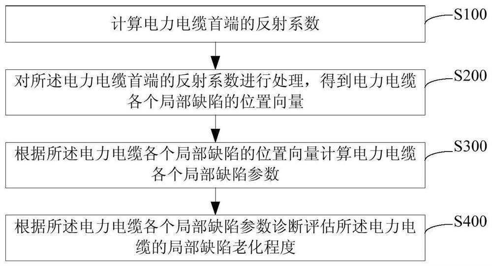
Local defect aging diagnosis and evaluation method for power cable
A technology for local defects and power cables, applied in the direction of measuring resistance/reactance/impedance, measuring electrical variables, instruments, etc., to reduce the amount of calculation, reduce the difficulty of calculation, and improve the probability of successful calculation
- Summary
- Abstract
- Description
- Claims
- Application Information
AI Technical Summary
Problems solved by technology
Method used
Image

Examples
Embodiment 1
[0107] The power cable to be tested in this embodiment is a 1000m ZR-YJV02 8.7 / 15 3*95mm2 power cable, and a resistor with an impedance of 1kΩ is connected in parallel at a position of 300m.
[0108] In this embodiment, an Agilent E5061B vector network analyzer is used to test the input impedance of the head end of the cable under test.
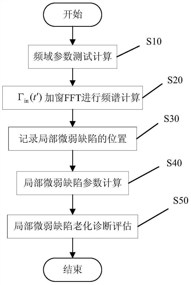
[0109] The local defect aging diagnosis method for power cables provided by this embodiment, such as figure 2 shown, including the following steps:
[0110] S10, frequency domain parameter test calculation
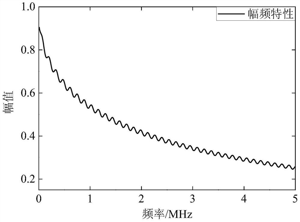
[0111] Set the sweep frequency range of the vector network analyzer to [10kHz, 5MHz], set the number of sweep points N to 1001 and set the input impedance Z at the head end of the power cable in (f) Conduct the test and then calculate the reflection coefficient Γ at the head end of the cable in (f):
[0112]
[0113] Calculated cable head end reflection coefficient Γ in (f) if image 3 shown. Where f is the scanning frequency p...
Embodiment 2
[0127] The power cable to be tested in this embodiment is a 1000m ZR-YJV02 8.7 / 153*95 mm2 power cable, and there is a local weak defect with a length of 1m at a position of 400m.
[0128] In this embodiment, an Agilent E5061B vector network analyzer is used to test the input impedance of the head end of the cable under test.
[0129] The local defect aging diagnosis method for power cables provided by this embodiment, such as figure 2 shown, including the following steps:
[0130] S10, frequency domain parameter test calculation
[0131] Set the sweep frequency range of the vector network analyzer to [10kHz, 5MHz], set the number of sweep points N to 1001 and set the input impedance Z of the cable head end in (f) Conduct the test and then calculate the reflection coefficient Γ at the head end of the cable in (f):
[0132]
[0133] Where f is the scanning frequency point; Z 0 It is the characteristic impedance measured by using a 10m long reference cable of the same mode...
PUM
 Abstract
Description
Claims
Application Information
PatSnap Eureka turns technology decisions into work you can execute. Powered by our Innovation Knowledge Graph, it runs expert workflows across engineering, life sciences, materials and intellectual property. Get your review-ready output in minutes.


