Flexible Huffman tree approximation for low latency coding

[0012] Overview

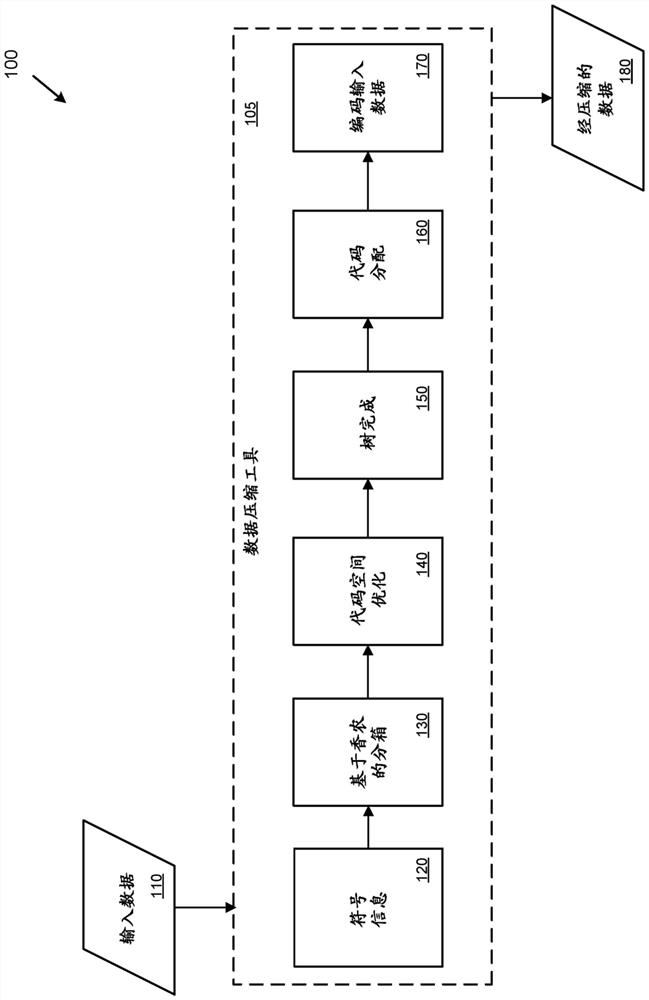
[0013] As described herein, various technical and technical solutions can be applied to approximate Hoffman coding algorithms (also known as Hoffmani algorithm, Huffman decoding or Hoffman code) without using Huffman coding. algorithm. For example, these techniques can be applied to encode (eg, compressed) data, which is close (eg, in one percent) Hoffman encoding but more efficient than Hofman coded (for example, in computing resources, delay) , Hardware implementation and other aspects of compression.

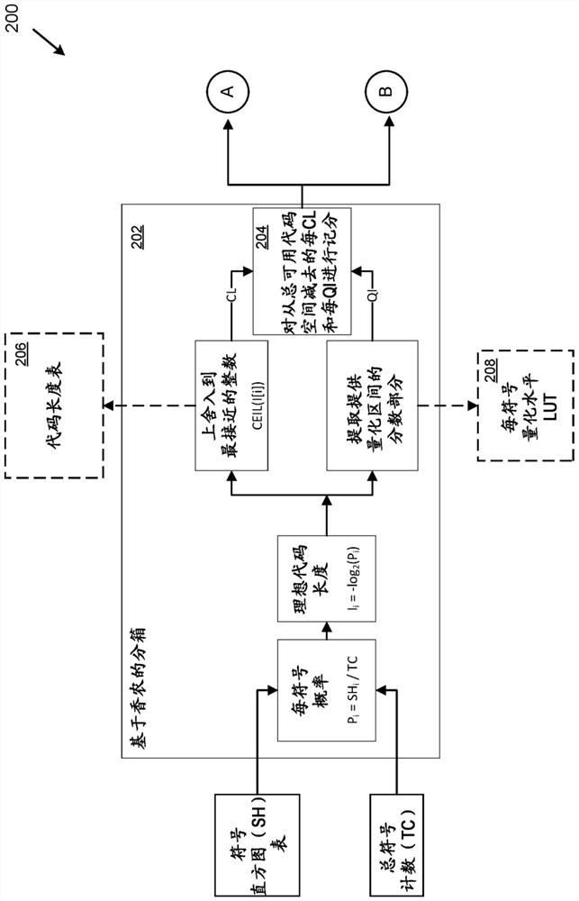
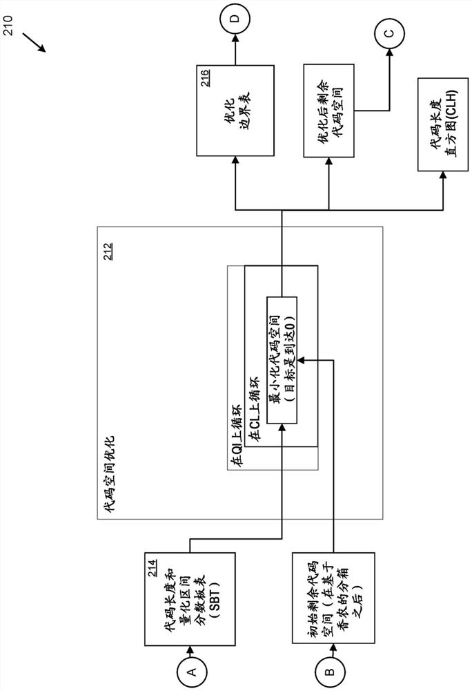
[0014] Techniques relate to a new algorithm for approximate Hofman algorithm. The new algorithm is also referred to as the quantization section Hofhman approximation (Quiha).

[0015] Depending on the implementation, the new algorithm can have one or more of the following properties:

[0016] * It produces a good compression ratio, which is usually within 0.05% encoded in True Hofman, which can be proven to be optimal.

[0017] * It is suitable for high-speed implementation of field programmable gate array (FPGAS) or dedicated integrated circuit (ASICS).

[0018] * For two-wheeled compression algorithm, it is an easy replacement of the Hofman algorithm and does not require a modification of the decompressor or compressed format specification.

[0019] The new algorithm can be applied to code symbols generated from input data. For example, the input data may be a file to be compressed, and data to be transmitted via the network, and the like. The input data can be any type of data (eg, text data, binary data, video data, audio data, etc.). The new algorithm is a lossless compression algorithm, where the symbols encode (eg, compressed) in a non-destructive manner. The new algorithm generates a symbol encoding a prefix code, and the code is 1 or more bit, similar to Huffman code. The prefix code is an item for encoding symbols using a variable length code.

[0020] For example, the new algorithm can be applied to the part of the encoding or compression process. For example, input data can be received (eg, data files, streaming, etc.). The input data can be processed to generate a symbol (e.g., as the initial stage of the DEFLATE compression algorithm, as a portion of the video or image encoder, etc.). Symbols (for example, including symbol counting and frequency information) can be processed by new algorithms (eg, including executing unannon-based box, code spatial optimization, tree completion, and / or execution of new algorithms), and code ( For example, the prefix code can be assigned based on the symbols being processed. The input data can then be output using code generated from the new algorithm (eg, a prefix code) in encoding or compressed format.

[0021] The new process is based on two basic implementations. First, a symbol having similar frequencies should be likely to be assigned with the same or similar code length. Therefore, the symbols can be organized into the biniqual based on the symbol frequency (further describing the Shannon-based biniqual process). Second, the symbol length assignment does not rely on the symbol ID them itself. Therefore, the count of the symbols in each split box can be used, not a list or collection of symbols, and the entire split box can be processed. The entire slider of the symbol is more efficient on the basis of the computing resource based on the symbol based on the symbol, as Hoffman coding.

[0022] The concept of the new algorithm introduces the code space. The code space covers all possible symbol encodings in a certain maximum code length constraint. For example, XPress8 (XPress8 is The supplied compression technology has a maximum code length of 15 bits, so the code space constraint 2 15 = 32K = 32,768 code for possible bit length 15. 1b (one) symbol uses half of the code (16K code), 2B (two) symbols use a quarter code (8K code), and so on. Table 1 below illustrates the code space used for each of the lengths of 15.

[0023]

[0024]

[0025] Table 1

[0026] In some implementations, the new algorithm is implemented in four phases. In the first phase (based on the Shannon Bank), the symbol is assigned to the initial code length based on the original fragrance algorithm. This algorithm may not make full use of code space and is not good to the Hofman algorithm. As symbols are processed, they are placed in the code length Box (CLB) based on their Shannon Code. The result is further improved by decomposing the CLB to quantify the interval (QI) based on the symbol frequency.

[0027] Since the first phase is not fully utilized, the subsequent code spatial optimization phase is substantially reducing the length of the code length by lifting some symbols from their initial CLB to the CLB, substantially reducing the length of the code length. This is the place where Qi is coming in. More optimized is shortening more frequently appearing symbols. By prioritizing the symbols in the most frequent QI, the algorithm achieves close to the optimal compression ratio.

[0028] The result of the code spatial optimization is quite good. However, the code spatial optimization phase is still an approximate heuristic type that may not make full use of code space. Some decompressors such as XPress8 require that the code space is completely dispatched, and it is equivalent to the symbol code tree is a full binary tree in which all of the parent nodes have two child nodes. The third stage, the tree is completed, the obtained tree is fixed and the slight improvement of the compression ratio can be obtained. These improvements are so slightly that this phase can be considered optional unless required by the decompression algorithm.

[0029] The final stage is the code allocation. The symbol is traversed and the actual prefix code is assigned. This phase follows the standard process in the case where the previously calculated code length of each symbol is given.

[0030] The following is an overview of some potential features of the new algorithm. Depending on the implementation, one or more of the features in the following features can be implemented.

[0031] * Approximate to the Hoffman algorithm, so that the slight reduction of the compression ratio is much reduced but a much higher hardware implementation.

[0032] * Symbol is sorted into the split box based on the symbol frequency. Assign the symbols in the same split box with the same / similar code length.

[0033] * Use simple scented scented code for initial code length estimation.

[0034] * The code length is further optimized based on the symbol frequency division.

[0035] * Further optimize the length of the code as necessary to complete the Hoffman tree.

[0036] Shannon-based box

[0037] In the techniques described herein, the Shannan-based binches are performed as part of the new algorithm. In some implementations, in the first phase of the new algorithm is performed in scented spoken boxes.

[0038] The new algorithm operates on the symbol. The symbol is received as an input to the new algorithm. Symbols can represent text (eg, character bytes) and / or other letters (eg, length, distance pair). In some implementations, the symbols are generated using the initial phase of the deflate compression algorithm. The initial stage of the DEFLATE compression algorithm is called Lemple-ZIF 77 (also known as LZ77). For example, the new algorithm can receive symbols from the initial phase of the DEFLATE compression algorithm and instead of executing Hoffman coding, the new algorithm uses the new algorithm technology described herein to encode symbols. In other implementations, the symbol uses another process (eg, from the initial phase of another compression algorithm).

[0039] Shannon-based binches are performed to determine the initial code length of the symbol and the symbol is placed in the corresponding code length Box (CLB) based on the initial code length assigned. In order to determine the initial code length, the equation 1 is used to calculate the length of the scented farmers. Then, the information content i () is rounded by the upper limit calculation according to equation 2.

[0040]

[0041] CLB (SYM) = CEIL (I (SYM)) (Equation 2)

[0042] In Equation 1, SYMCNT [] is the number of occurrences of each symbol, and Symtot is the total number of symbols in the input (e.g., the total number of symbols generated by the input file to be compressed by the initial phase of the deflate compression algorithm). Note that the symbols that have not occurred (Symcnt [SYM] == 0) does not require code assignment and can be skipped.

[0043] In some hardware implementations, SYMCNT and SYMTOT are instantly calculated during the LZ77 phase. As each symbol is generated, Symtot and Symc [SYM] are added. The histogram of the symbols is therefore available to the start of the build symbol table.

[0044]For example, Xpress8 compressed format uses 512 symbols (ie, 512 9-bit symbols). Therefore, using XPress8, SYMCNT [] contains the number of occurrences of each symbol in 512 symbols in input data to be compressed. Other compressed formats can use different quantities of symbols.

[0045] The number of code length splits corresponds to the maximum code length of the compressed format being used. For example, the XPRESS8 compressed format has a maximum code length of 15 bits. Therefore, when using XPress8, there are 15 CLBs, one for 1 bit code, one for 2-bit code, one for 3-bit code, and so on. In some implementations, you can use a length of code below the maximum code length. For example, if the compressed format does not have a strict limit or a more efficient implementation, a lower code length can be used.

[0046] The allocated CLB for a given symbol represents the initial symbol length in bits. In some implementations, the new algorithm keeps tracking the remaining code space (eg, after assigning the symbol to the CLB). The code space is defined by the maximum code length used. For example, for XPress8, the maximum code length is 15 bits, and the code space is 32,768 (which is the maximum available code space, and the maximum number of code is indicated when all code is 15 digits). The remaining code space can be tracked using equation 3.

[0047] REM_CODE_SPACE- = 2 maximum_code_length-CLB(sym) (Equation 3)

[0048] The remaining code space (REM_CODE_SPACE or RCS) is initialized to the maximum code space, which is 32, 768 in this example. Skilon code is of course justified to implement code, which guarantees that REM_CODE_SPACE will not become negative. The remaining code space is then updated when the symbol is assigned to the CLB. For example, if the symbol is assigned to 6-bit CLB, the remaining code space is updated: REM_CODE_SPACE = 32, 768-512 = 32, 256. If the symbol is then assigned to 4-bit CLB, the remaining code space is updated: rad_code_space = 32, 256-2, 048 = 30, 208.

[0049] In some implementations, each CLB is divided into a plurality of quantization ranges (QI). Each QI represents a continuous portion of the information content for each CLB. More specifically, the fractional portion of the information content is divided into QI. In some implementations, the fractional portion is equal to many QIs. In some implementations, the fractional portion can be divided into four QIs using equation 4.

[0050] Qi (SYM) 3-FLOOR ((CLB (SYM) -i (SYM)) * 4) (Equation 4)

[0051] QI 0 contains the most frequent symbols for a given CLB, and QI 3 contains the least frequent symbols for a given CLB. In other implementations, different numbers of QIs can be used, or can be used (e.g., except for the equal-equivalent partial division fractional portion). Different processes.

[0052] During the Shannon-based split box, the count can be maintained for the number of symbols assigned to each CLB and / or each QI. In some implementations, only counts of only count-based spinning boxes are assigned to each of each of each of the QIs in the CLB. For example, if there are 15 CLBs, each having four QIs, then 60 counts can be maintained (eg, a count array of 15x4).

[0053] Code spatial optimization

[0054] In the techniques described herein, code spatial optimization is performed as part of a new algorithm. In some implementations, the code spatial optimization is performed in the second phase of the new algorithm. The code spatial optimization is performed to shorten the symbol to a shorter code length box (eg, from a given B bit CLB to B-1 CLB). For example, symbols can be shortened by moving symbols from 6-bit CLB to 5-bit CLB (which is the next shorter code length split box) (also known as "lifting"). For example, code spatial optimization can be performed, as scented-based split boxes can produce unsuitable code space.

[0055] In some implementations, the code spatial optimization is determined (for example, if the remaining code space is maintained during the Shannon-based split box) is executed. If the remaining code space is equal to zero, the code spatial optimization can be skipped (for example, the code space has been fully utilized and no symbol needs to be moved).

[0056] In some implementations, the remaining code space is updated during the code spatial optimization. For example, when the symbol is moved to the next smaller CLB, the remaining code space is updated according to equation 5. Code spatial optimization can proceed until the remaining code space is close or equal to zero.

[0057] REM_CODE_SPACE- = 2 max-b (Equation 5)

[0058] In Equation 5, max is the maximum code length (for example, for xPress8, 15) and "b" is the number of bits we are moving from it. For example, if we are moving symbols from 6-bit CLB to 5-bit CLB, then the remaining code space will be subtracted 512.

[0059] In some implementations, the code spatial optimization is performed by first lifting symbols in the most frequent QI. For example, Qi 0 can be traversed (2-bit CLB; CLB 1 cannot be shortened) in all CLBs starting at CLB 2; For each QI, as many symbols as possible can be shortened so that the code space is not excessive (e.g., maintained by the remaining code space). The following algorithms can be used to shorten symbols in QI and CLB.

[0060]

[0061] Note that Reduction_Per_SYM is always the power of the second, and can be represented only by an index rather than the integer as shown. The division becomes right shift, and the multiplication becomes left shift. As a performance optimization, the cycle can be terminated when the REM_CODE_SPACE is zero. Additional place, once REM_CODE_SPACE <2 (15-clb) There is no need to reconsider the low-numbered CLB.

[0062] Lift symbol (Shortensymbols (...) is only involved in recording how many symbols have been shortened. If all the previous smaller numbered QIs have been completely shortened, the larger number of QIs can have only shortened symbols. This is because the only thing that will prevent the previous QI completely shortened is the remaining code space, which is similarly limited to the later QI.

[0063] As a result, the number of shortening symbols per Qi does not need to be tracked. Instead, this can be accomplished using two fields per CLB. The first field maxShortenedQi [CLB] indicates the largest (least frequent) QI with a shortened symbol. The second field Symshortened [CLB] indicates how many symbols in the QI are shortened. All QIs smaller than maxshortenedqi are completely shortened. All QI greater than maxshortenedqi does not have a shortened symbol.

[0064]

[0065] Tree completion

[0066] In the techniques described herein, the tree completion can be performed as a new algorithm. In some implementations, the tree is completed is an optional phase. For example, the Shannon-based box and code spatial optimization phase can still make the code space completely (when being represented as a binary tree structure). In other words, the remaining code space can still be non-zero. The code tree interpretation is that the binary tree may not be a binary but contain a parent node with only one child node. Note that all Hoffmanows is a binary tree. Some decompressors can contemplate the nature of the node. It is important to keep in mind that the binary tree is not necessarily Hoffman (optimal) tree. However, all Hoffmanows is a binary tree.

[0067] The tree completion phase promotes lower nodes in the tree to higher levels (lower length), so the higher empty child nodes in the tree are filled. The algorithm processes the trees of any shape, but some constraints can be observed and utilized for efficient hardware implementation. For example, you can apply empty The constraints can be on any hierarchy of the tree in addition to the first level (length 1).

[0068] In some implementations, the tree completes only the code length of the symbol, without considering the corresponding QI. Moreover, the tree completion can reduce the symbol to one bit to reduce the remaining code space (RCS) faster than zero. The tree is completed on the code length histogram (CLH) (which is an accumulated view of the QIPOP of QIPOP). Conceptually, the tree completes binary representation of RCS representing node vacancy and surplus of nodes in binary codes. The output of the tree includes tracking the code length scoreboard (CLSB) of the FROM-TO node to facilitate the count. CLSB is used in the final code assignment phase to shorten the code length of the symbol.

[0069] In some implementations, the operation below is performed for the tree:

[0070] Abundance on CLH until RCS! = 0

[0071] 1. Get the MSB of RCS to provide the result of Floor (RCS); this is a long-length symbol will be an upgrade length TO; if the RCS is 2 power and corresponds to the CLH of the TO (purpose) code length The entry is greater than 0, then the length is reduced; the length corresponds to a tree level having a node shortage.

[0072] 2. Reduce the RCS to the code space obtained by a single symbol at the length of TO.

[0073] 3. Increase the CLH entry of the TO length.

[0074] 4. The obtained symbol will be removed from the surplus length from; this is determined by the LSB of the updated CLH having a constraint of the FROM length> TO length; the length corresponds to the tree level of the surplus node.

[0075] 5. Reduce the CLH entry of the future.

[0076] 6. Update CLSB to explain the upgrade.

[0077] In some implementations, the tree completion phase fills any missing nodes to make the code space are represented as a full bifurcation.

[0078] Code assignment

[0079] In the techniques described herein, the code allocation is executed as a part of the new algorithm. In some implementations, the code is allocated in the final phase of the new algorithm (eg, the third phase or fourth stage, depending on whether the tree is completed, is executed). During the code allocation, the last code length for each symbol can be calculated by recalculating the CLB and Qi and is followed by each QI adjustment information. The code allocation can be performed by using a Hoffman algorithm (for example, a paradigm-Hoffman coding algorithm or another Hoffman variant) in the case of a bitmier for each symbol.

[0080]In some implementations, the number of symbols per length is maintained immediately by the previous stage. Therefore, this information is known in the start of the code allocation, and there is no clear reciprocation of the symbol. This information is given, the code space is divided by code length, thereby initializing each code pointer (ie, first code) (ie, first code) (or using a different number of possible code lengths) for 15 possible code lengths, depending on Compression format). For each symbol, its code length is recalculated as described herein (eg, as described at 232), and it is assigned to the current code pointer for its length. The code pointer is then updated to the next code.

[0081] Example block diagram

[0082] figure 1 A block diagram 100 depicting an example process for encoding data using a new algorithm to achieve a flexible Hofman tree approximate. Operations performed by the example process are generally described as data compression tools 105. However, these operations can be performed by various combinations of software and / or hardware resources.

[0083] In box figure 1 In, the input data 110 is received. The input data 110 can be any type of data (eg, text data, binary data, video data, audio data, etc.). At 120, symbol information is generated from the received input data 110. Symbol information can include symbol counting and frequency information. In some implementations, the symbol information is generated by using the LEMPLE-ZIF 77 (also known as the LZ77) algorithm (for example, as the initial phase of the DEFLATE compression algorithm).

[0084] At 130, a sponsors based on scented. Shannon-based binches are performed to determine the initial code length for symbols and place symbols in the corresponding code length splitter based on the initial code length of the symbol. In some implementations, each CLB is divided into many QIs. Each QI is based on the Shannon code length to represent the continuous portion of the CLB.

[0085] At 140, the code spatial optimization is performed. The code spatial optimization is performed to shorten the symbol to a shorter code length box.

[0086] At 150, the execution tree is completed. In some implementations, the tree is completed is an optional phase. The tree completes the lower node to higher level (lower length) in the tree, so the higher "empty" in the trees.

[0087] At 160, the code assignment is executed. During the code allocation, the final code length for each symbol can be calculated (e.g., by recalculating the CLB and Qi, and following each qi adjustment information). Using symbol information, the prefix code can be generated for encoding input data 110. In some implementations, the prefix code is generated based on the code allocation section of the Hoffman coding algorithm (eg, according to the code allocation section of the paradigm Hofman coding algorithm).

[0088] At 170, the input data 110 is encoded using the code assigned at 160. The encoded data is outputted as a compressed data 180.

[0089] In some implementations, one or more of the operations depicted in block diagram 100 are implemented in hardware. For example, hardware components (eg, ASIC or FPGAs) can implement some or all of the operations as part of the data compression process.

[0090] In some implementations, block diagram 100 is implemented as part of a cloud computing service. For example, the cloud computing service can provide a data storage service. One or more of the operations depicted in block diagram 100 can be used to compress data when data is stored by data storage services.

[0091] In some implementations, block diagram 100 is implemented as part of a network data compression tool. For example, a source device (eg, a desktop or laptop, server, smart phone, or another type of computing device) or network device (eg, router, gateway, firewall, switch or another type of network device) can via The computer network receives input data for transmission and compresses input data using some or all of the operations described in block diagram 100. Compressed data can be unzipped by subsequent network devices or devices (eg, desktops or laptops, servers, smart phones, or other types of computing devices), or it can be stored in their compression format (for example At the destination device).

[0092] Example advanced operation block diagram

[0093] Figures 2A-2D Example advanced operation block diagram depicting the flexible Hoffman approximation algorithm. The block diagram depicts many implementation details that may or may not be used in a particular implementation. For convenience, the block diagram depicts an example implementation of a new algorithm for 15-bit maximum code lengths (and 15 CLBs) (with up to 512 symbols), and four quantitative intervals (4 QIs) are used. Other implementations can have different maximum code lengths, different quantities of symbols, and / or different quantization ranges. The following symbols are followed in Figures 2A-2D Example implementation in the depiction:

[0094] SH: Symbol histogram (also known as Symcnt [])

[0095] SH [I]: Symbol I of symbol I.

[0096] TC: The total symbol count (also known as symtot)

[0097] Qi: quantization range

[0098] CL: Code length (also known as CLB)

[0099] SBT: Scoreboard table (also known as QIPOP)

[0100] OBT: Optimize Boundary Table

[0101] CLH: Code length histogram

[0102] CLSB: Code length scoreboard

[0103] RCS: Remaining code space (also known as REM_CODE_SPACE)

[0104] FBT: Full Binary Tree

[0105] Generally, the stage of the new algorithm is depicted in block diagram in the order from left to right. Figure 2A A first portion 200 depicting a block diagram of the implementation of the universal binoculation phase 202 is depicted. In the Shannon-based split box phase 202, the algorithm is iterated on all histogram entries, thereby generating the length of the scented scented scented scented scented scented scented scented scented scented scenario and score each code length and each quantitative interval. The remaining code space is also legged in the histogram (e.g., according to equation 3) to obtain remaining code space for subsequent optimization steps.

[0106] Based on the Shannon Box Phase 202 generally performs the operation corresponding to those discussed above with respect to Equation 1 and 2 to determine the initial code length. Based on Shannon's Box Phase 202 is also divided into quantization intervals based on the fractional part of Shannon Code (for example, according to equation 4). The score (count) is maintained for each code length splitter and each quantization section, as depicted at 204. For example, a table containing symbol distributions on Cl and Qi can be created.

[0107] The fractional part of the Xiangnong code length is divided into QI. In some implementations, the fractional portion is divided as depicted in Table 2. Note that the fractional portion of 0 is mapped to the last (lowest priority) QI, because the symbol is not optimized when its ideal code length is integer.

[0108]

[0109]

[0110] Table 2

[0111] The code length table 206 (CLT) (which is 512 multiplied in this example) includes an integer part of the ideal code length used as the baseline code length. It is the first optimization priority. In some implementations, maintaining CLT is optional, such as indicated by a broken line (for example, the length of code can be recalculated at the code assignment phase).

[0112] The quantization range of the second optimization priority of the code indicating the symbol is included in the example (which is 512 multiplied in this example) contains a second optimization priority of the code indicating the symbol. In order to save storage resources, each symbol quantization section LUT can be re-calculated at a later stage later. In some implementations, it is optional, such as indicated by a broken line (for example, the quantization section can be recalculated at the code assignment phase).

[0113] Figure 2b A second portion 210 depicting the implementation of the block diagram of the description code spatial optimization phase 212 (which is also referred to as a code length optimization).

[0114] As depicted at 214, the code length and quantization section score sheet (SBT) are maintained. The SBT can contain 15x4 entries. SBT provides a length optimization priority per code.

[0115] In some implementations, the code spatial optimization phase 212 uses two nesting loops to process SBT, the first in Qi, after the length of the code, both in ascending (priority). At each step, the optimizer calculates that the symbol of them can reduce the number of remaining code spaces to become negative symbols, and the optimization target is accurate to 0, which depends on the symbol distribution is not always possible. In this way, the optimizer effectively compresses the code tree.

[0116] As depicted at 216, an optimized boundary table (for example, 15 entries) is generated. Each CL optimization boundary table includes QI and indication how many symbols can be optimized at the corresponding QI of all the same CL symbols, where higher priority QI is implied.

[0117] Figure 2C A third portion 220 that depicts the implementation of the block diagram of the tree completion phase 222. The tree completion phase 222 generates a bifurcous tree, which implies zero remaining code space. The tree completion phase 222 includes a code length adjustment sub-stage 224 that decreases the symbol length based on the symbol ascending in the CLT, based on the CL / QI assignment from the OBT to reduce the symbol length. The code length adjustment sub-stage 224 also constructs a CL histogram (CLH) that tracks the symbol code length distribution of the strict binary tree properties (which has 15 entries in this example). In some implementations, the code length adjustment sub-stage 224 is optional.

[0118] The tree completion phase 222 includes a bifurcous (FBT) sub-stage 226 that itself is iterated by two times on the length histogram, using the remaining code space binary representation to guide the length (symbol upgrade) at each iterative step (symbol upgrade), so that the remaining The code space is 0. In some implementations, the full bifurcation (FBT) sub-stage 226 performs the following stage:

[0119] When the remaining code space (RCS)> 0

[0120] - Gets the MSB of RCS to provide Floor (LOG2 (RCS)); this is the length TO of higher length symbols will be upgraded; if RCS is 2 power and corresponds to the CLH entry of the TO (purpose) code length More than 0, then minus 1

[0121] - Update RCS, CLH, CLSB to explain the upgrade; CLSB tracks the symbol count shorting / surplus per code length

[0122] - The surplus length from the obtained symbol will be removed; this is determined by the LSB of the updated CLH with the constraint of the from the length> TO length.

[0123]The tree completion phase 222 includes a generating an adjacent matrix (AM) sub-stage 228 that converts it twice in CLSB, thereby converting it into a hardware optimized quick lookup table used as an adjacency matrix of the extension of the from-TO symbol. At most 2 symbols can be upgraded from one length to another.

[0124] Figure 2D A fourth portion 230 of the implementation of the description code assignment phase 232 of the block diagram is depicted. The code assignment phase 232 follows the paradigm Huffman code book generation algorithm, except that it instantly executes the length of the symbol.

[0125] The code assignment phase 232 includes establishing a first codon phase 234 per length that is heated on the CLH according to the length of the length, thereby generating a first code for each length based on the length of the histogram scale. The first code (which includes 15 entries in this example) is provided to the codon phase 236 that sets each symbol. The code sub-stage 236 of each symbol is provided with iteration on all symbols according to the ascending order, thereby adjusting the length of each of the AMs and assigns the code according to the final CL of each symbol. In some implementations, the codon phase 236 of each symbol is set to use the code length table 206 generated earlier. In other implementations, the codon phase 236 of each symbol is set to recalculate the initial code length and quantization range, as according to the Shannon's Box Phase 202 (but does not perform a split box), and recalculate the code length, such as settings The operation of the code sub-stage 236 of each symbol is depicted.

[0126] The code assignment phase 232 code is assigned to the symbol based on the encoding algorithm being used. In this implementation, the code assignment phase 232 generates paradigm Hoffman code to output.

[0127] Method for encoding symbols using flexible Hoffman tree

[0128] In any example of this article, it is possible to provide a method for encoding symbols using a new algorithm to achieve an approximate Hoffman tree.

[0129] image 3 It is a flow diagram of an example method 300 for encoding symbols using a new algorithm. For example, the example method 300 can be executed by a computing device (e.g., software running on a computing device) and / or by a hardware component of a computing device (eg, by an ASIC for FPGA).

[0130] At 310, a sponnar-based split box is performed to determine the initial code length of the symbol and the symbol is placed in a corresponding code length Box (CLB) based on the assigned initial code length. Shannon-based bins can be performed as part of the first phase of the encoding process. In some implementations, the CLB is divided into quantization ranges. In some implementations, the symbols are received from another compression or encoding tool, such as receiving a tool using a deflate compression algorithm. For example, data to be compressed can be received (e.g., as a file, as stream data, or in another format). The data can be processed to generate symbol information, which can be provided to input to the example method 300.

[0131] At 320, the code spatial optimization is performed to shorten at least some of the symbols to a shorter code length box. For example, the lifting symbol can be performed based on the amount of the remaining code space. Code spatial optimization can be performed as a part of the second phase of the encoding process. In some implementations, the code spatial optimization is performed when the remaining code space is greater than the threshold (for example, when the code space is greater than zero). For example, if the remaining code space is less than or equal to the threshold, the code spatial optimization can be skipped.

[0132] At 330, the tree is completed by transitioning the binary tree into a binary tree by a binary tree of the symbol. In some implementations, the tree is not executed (for example, the tree is completed can be an optional phase).

[0133] At 340, the prefix code is assigned to the symbol based at least in part on the code length bin. In some implementations, the prefix code is assigned based on the code allocation section of the Hoffman code algorithm (eg, according to the code allocation section of the paradigm Hoffman coding algorithm).

[0134] Figure 4 It is a flow diagram of an example method 400 for encoding symbols using a new algorithm. For example, example method 400 can be executed by a computing device (e.g., software running on a computing device) and / or by a hardware component of a computing device (e.g., by an ASIC for FPGA).

[0135] At 410, the symbol information is received. Symbol information is generated from input data (eg, input files, stream data, etc.). The symbol information includes symbols and frequency information generated from input data. In some implementations, the symbol information is generated from a compression algorithm (eg, using the LZ77 algorithm).

[0136] At 420, the incense-based split box is performed to determine the initial code length of the symbol and the symbol is placed in a corresponding code length Box (CLB) based on the assigned initial code length. Shannon-based bins can be performed as part of the first phase of the encoding process. In some implementations, the CLB is divided into quantization ranges.

[0137] At 430, the code spatial optimization is performed to shorten at least some of the symbols to a shorter code length box. For example, the lifting symbol can be performed based on the amount of the remaining code space. Code spatial optimization can be performed as a part of the second phase of the encoding process. In some implementations, the code spatial optimization is performed when the remaining code space is greater than the threshold (for example, when the code space is greater than zero). For example, if the remaining code space is less than or equal to the threshold, the code spatial optimization can be skipped.

[0138] At 440, the tree is completed by transitioning the binary tree into a binary tree by a binary tree of the symbol. In some implementations, the tree is not executed (for example, the tree is completed can be an optional phase).

[0139] At 450, the prefix code is assigned to the symbol based at least in part on the code length bin. In some implementations, the prefix code is assigned based on the code allocation section of the Hoffman code algorithm (eg, according to the code allocation section of the paradigm Hoffman coding algorithm).

[0140] At 460, the input data is encoded using the assigned code (eg, using the assigned Hoffman code). The encoded input data (which is now in a compressed format) can be output (e.g., as the compressed file is saved on the storage device, as the compressed data stream is sent to network devices, etc.).

[0141] Integer implementation

[0142] The new algorithm can be implemented using an integer implementation (eg, hardware, such as ASICS, and FPGAS).

[0143] Register Transfer Level (RTL) implementation should avoid high cost and inaccurate floating point calculations, especially log2 and division. In addition, the CLB must not be less than the precise value, or the code space may overflow, resulting in incorrect functionality. In order to solve these potential problems, efficient and accurate integers have been developed using the following variations.

[0144] CLB (SYM) = CLB

[0145] CEIL (I (SYM)) = CLB

[0146] CLB-1

[0147] CLB-1

[0148] CLB-1

[0149] 2 clb-1

[0150] 2 clb-1 * SYMCNT [SYM] clb * SYMCNT [SYM]

[0151] 2 clb * SYMCNT [SYM] clb * SYMCNT [SYM]

[0152] 2 clb * SYMCNT [SYM]

[0153]

[0154] Symtot clb * SYMCNT [SYM]

[0155] The CLB can be calculated by first aligning the high order of Symcnt [SYM] with the Hue of Symtot and then compares Symtot. The number of digits will be referred to as CLB '.

[0156] CLB = CLB'IF Symtot clb′ * SYMCNT [SYM]

[0157] CLB = CLB '+ 1 2HERWISE

[0158] QI is optimized, and accurate calculations will not affect the correctness. Qi is calculated using the cut point between Symtot and 2 * Symtot. The cutting point is calculated once in front. In this implementation, simple linear cutting points are used, but from the perspective of information theory, the log-based mode is more accurate. The following QI cutpoints depicted in Table 3 will be used in this implementation using four QI, and the following QI cutting points depicted in Table 3 are used in this implementation.

[0159]

[0160] Table 3- Quantifier Interval Border

[0161] In this way, QI can also calculate an integer operation. It is not critical when calculating the boundary point.

[0162] Hardware implementation

[0163] The new algorithm can be implemented efficiently with hardware (such as ASICS and FPGAS). For example, the technology can implement parallel calculations of multiple symbols. The number of symbols processed per cycle will depend on factors such as chip area constraints, target frequencies, and technologies being used. Common implementations can process up to 4 symbols per cycle. SYMCNT can be implemented, for example, by arrays and SRAM during spoken boxes based on Shannon. Since access to the symbol count is the order, multiple symbols continuous count can be readily read. Calculation of CLB and Qi is completely independent of each symbol, so multiple symbols can be handled in parallel.

[0164] Updates to QIPOP involve simple logic and increase. The multiple increase in the same entry can be combined into a single addition, thereby allowing multiple symbols to be scaled in parallel.

[0165] Code spatial optimization cycle (for example, Figure 2b The 212 depicted in 212 is serialized on the update to the RCS. Therefore, each iteration is processed once. Therefore, each iteration of the circulation 212 is serialized. However, the cycle can be reduced to a simple integer operation, usually implemented in a single cycle. In addition, the code spatial optimization will usually run only several iterations.

[0166]The code allocation involves the second round of symbols. Multiple symbols can calculate their final code length: 1) Read symbol count and calculate the CLB and Qi, 2) of Shannon, and apply OBT CLB updates from code space optimization, and 3) parallel. Apply the AM update tree completion, and 4) to allocate the code based on the FCT. As in the spoken box based on scented, the symbol count, CLB and Qi can usually read and calculate in parallel using the same hardware pipeline. Updates to OBT can be optimized by combining updates to multiple symbols when multiple symbols have the same CLB and QI, allowing multiple symbols to be processed at a single cycle. Similarly, an update to the AM can be merged when multiple symbols have the same CLB (after OBT adjustment). This produces the final code length for multiple symbols at each cycle.

[0167] In the end, the code is allocated by consulting the FCT based on the final code length. When multiple symbols have the same final code length in the same period, they can be combined with the update of the FCT, thereby converting multiple adds into a single small phase plus. This gets the final assigned code for multiple symbols at each cycle.

[0168] Computing system

[0169] Figure 5 A general example of the appropriate computing system 500 described in the described technique can be implemented. Computing system 500 is not intended to imply any restrictions on the scope or function because these techniques can be implemented in a wide variety of general or dedicated computing systems.

[0170] refer to Figure 5 The computing system 500 includes one or more processing units 510, 515, and memory 520, 525. exist Figure 5 In the basic configuration 530 being included in the dashed line. Processing units 510, 515 run the computer executable instruction. The processing unit can be a general-purpose central processing unit (CPU), a processor in a dedicated integrated circuit (ASIC) or any other type of processor. The processing unit can also include a plurality of processors. In multiprocessing systems, multiple processing units run computer executable instructions to improve processing capabilities. E.g, Figure 5 The central processing unit 510 and a graphics processing unit or a synergistic processing unit 515 are shown. The shapes of memory 520, 525 may be volatile memory (e.g., registers, cache, RAM), non-volatile memory (e.g., ROM, EEPROM, flash memory, etc.) or both by (multiple) processing units. Specific combination. Memory 520, 525 stores software 580 of one or more techniques described herein in the form of a computer executable instruction suitable for operation by (plurality) processing units.

[0171] The computing system can have additional features. For example, computing system 500 includes storage device 540, one or more input device 550, one or more output devices 560, and one or more communication connection 570. An interconnect mechanism such as a bus, a controller, or a network (not shown) interconnects the components of the computing system 500. Typically, the operating system software (not shown) provides an active environment for operating an operating environment for other software in computing system 500 and coordinating component 500 components.

[0172] The shapeless storage device 540 can be removable or not removable, and include a disk, a tape or cartridge, a CD-ROM, a DVD, or any other medium that can be used to store information and can be accessed within computing system 500. The storage device 540 stores instructions for implementing software 580 of one or more techniques described herein.

[0173] (Multiple) The input device 550 can be a touch input device such as a keyboard, a mouse, a pen, or a trackball, a voice input device, a scanning device, or another device that provides input to the computing system 500. For video encoding, (multiple) input device 550 can be a camera, video card, a TV tuning card, or a similar device accepted by video input in analog or digital form, or read video samples into the CD in the computing system 500. -ROM or CD-RW. (Multiple) The input device 560 can be a display, a printer, a speaker, a CD burner, or another device supplied from the output from the computing system 500.

[0174] (Multiple) Communication Connections 570 implements communication through communication media to another calculation entity. The communication medium communicates information such as a computer executable instruction, audio or video input or output, or other data. The modulation data signal is a signal that is set or changed in a manner that encodes information in the signal. By way of example, the communication medium can use electrical, optical, RF or other carriers.

[0175] These techniques can be operated in the computer executable instructions such as those included in the program module), run on the target real or virtual processor on the computing system. In general, program modules include routines, programs, libraries, objects, classes, components, data structures, and more to perform specific tasks or implement specific abstract data types. In various embodiments, the function of the program module can be combined or split between the program module as needed. Computer executable instructions for program modules can be run within the local or subsequent layout computing system.

[0176] The term "system" and "equipment" are used interchangeably herein. Unless the context is clearly indicated separately, any of the terms of a type of computing system or computing device is implied. Generally, the computing system or computing device can be local or distributed, and may include a dedicated hardware and / or universal hardware and any combination of software implemented herein.

[0177] To show, a terminology using as "OK" and "Use" is described in detail to describe computer operations in the computing system. These terms are advanced abstractions for operations performed by a computer, and should not be confused with the action performed by the human being. The actual computer operation corresponding to these terms varies depending on the implementation.

[0178] Cloud support environment

[0179] Image 6 It is a generalized example of the described embodiments, techniques, and processes that can be implemented in the appropriate cloud support environment 600. In the sample environment 600, various types of services (eg, computing services) are provided by the cloud 610. For example, cloud 610 can include some computing devices, which may be centrally positioned or distributed, which provides cloud-based services to various types of users and devices connected via networks such as the Internet. Implementation Environment 600 can be used in different ways to complete the computing task. For example, some tasks (eg, processing user inputs and presentation user interfaces) can be performed on local computing devices (e.g., connection devices 630, 640, 650), while other tasks (storage to be used in subsequent processing) It can be performed in the cloud 610.

[0180] In the sample environment 600, the cloud 610 provides a service for connection devices 630, 640, 650 with various screen capabilities. Connection device 630 denotes a device having computer screen 635 (eg, a medium-size screen). For example, the connection device 630 can be a personal computer, such as a desktop computer, a laptop, a notebook, a netbook, and the like. The connection device 640 represents a device having a computer screen 645 (eg, a small size screen). For example, the connection device 640 can be a mobile phone, a smart phone, a personal digital assistant, a tablet computer, and the like. The connection device 650 denotes a device having large screen 655. For example, the connection device 650 can be another device such as a television screen (e.g., smart television) or a television (eg, a top box or a game console). One or more of the connecting devices 630, 640, 650 can include touch screen capabilities. The touch screen can be accepted in different ways. For example, the capacitive touch screen detects the touch input when the object (eg, a fingertip or stylus) is distorted or interrupt. As another example, the touch screen can detect the touch input when the optical sensor is interrupted when the light beam from the optical sensor is interrupted. Physical contact with the surface of the screen is not necessary for inputs to be detected by some touch screens. Devices without screen capabilities can also be used in the sample environment 600. For example, cloud 610 can provide services for one or more computers (eg, server computers) without a display.

[0181] The service can be provided by the cloud 610 via the service provider 620 or other provider (not depicted) through the online service. For example, the cloud service can be customized depending on the screen size of a particular connection device (eg, connection devices 630, 640, 650), display capabilities, and / or touch screen capability.

[0182] In the example environment 600, the cloud 610 is at least partially supplied to various connection devices 630, 640, 650 using the service provider 620. For example, service provider 620 can provide a centralized technical solution for a variety of cloud-based services. Service provider 620 can manage service subscriptions for users and / or devices (e.g., users for connecting devices 630, 640, 650, and / or their respective).

[0183] Example implementation

[0184] Although some of the operations disclosed are described in order to facilitate the presentation, such a description manner includes rearrangement, unless a specific order is required by the particular language required by the following. For example, the operations described in order can be rearranged or concurrently in some cases. Furthermore, for simplicity, the drawings may not show various ways to be used in conjunction with other methods.

[0185] Any method in the disclosed method can be implemented to be stored on one or more computer readable storage media and run on a computing device (ie, any available computing device, including smartphone or other mobile device including computing hardware). Computer executable instructions or computer program products. Computer readable storage media is a tangible medium (one or more optical media discs, such as DVD or CDs, volatile media, such as DRAM or SRAM) or non-volatile media (such as flash memory or hard disk) or non-volatile media (such as DRAM or SRAM) (such as DRAM or SRAM) (such as DRAM or SRAM) or non-volatile media (such as DRAM or SRAM) or non-volatile media (such as flash memory or hard disk) driver)). By way of example and reference Figure 5 The computer readable storage medium includes memories 520 and 525 and storage device 540. The term computer readable storage medium does not include signals and carriers. In addition, the term computer readable storage medium does not include a communication connection, such as 570.

[0186] Any data used to implement the computer executable instructions disclosed in the disclosed technology and any data created and used during the implementation of the disclosed embodiments can be stored on one or more computer readable storage media. Computer executable instructions can be part of the dedicated software application or software application access or downloaded via a web browser or other software application (such as remote computing application). Such software can be run, for example, on a single local computer (e.g., any suitable commercial computer) or a network environment using one or more network computers (eg, via the Internet, WAN, LAN, and Client Server network (such as cloud computing network) ) Or other such networks).

[0187] In order to clear, only some of the selected aspects of software-based implementation are described. Other details well known in the art will omit. For example, it should be understood that the disclosed techniques are not limited to any particular computer language or program. For example, the disclosed technique can be implemented by software written in C ++, Java, Perl or any other suitable programming language. Similarly, the disclosed techniques are not limited to any particular computer or type of hardware. Some details of the appropriate computer and hardware are well known and unquestied in the present disclosure.

[0188]In addition, any embodiment of the software-based embodiment (including, for example, computer executable instructions for making a computer in the disclosed method) can be uploaded, downloaded or remotely accessed by the appropriate communication means. Such appropriate communication methods include, for example, internet, web, intranets, software applications, cables (including fiber optic cables), magnetic communication, electromagnetic communication, electronic communication, or other such communication means .

[0189] The methods, apparatus, and systems disclosed are not to be construed as limiting. Alternatively, the present disclosure points to all novel and non-apparent features and aspects of various disclosed embodiments, individually and in combination with each other. The disclosed methods, apparatus, and systems are not limited to any particular aspect or feature or a combination thereof, and the disclosed embodiments do not require any one or more specific advantages or problems to be resolved.

[0190] Techniques from any example can be combined with the techniques described in any one or more of other examples. In view of the various possible embodiments of the disclosed techniques, the illustrated embodiments are illustrative of the disclosed techniques and should not be construed as limiting the scope of the disclosed techniques.