System for geometrically accurate compression and decompression
a compression and decompression system technology, applied in the field of system for compressing and reconstructing signals, can solve the problems of large errors in derived quantities obtained from reconstructed data, inaccurate reconstruction of terrain features, and large errors in determining gradients from reconstructed data, so as to achieve accurate compression and reconstructed gradients, accurate reconstruction, and accurate reconstruction
- Summary
- Abstract
- Description
- Claims
- Application Information
AI Technical Summary
Benefits of technology
Problems solved by technology
Method used
Image
Examples
example 1
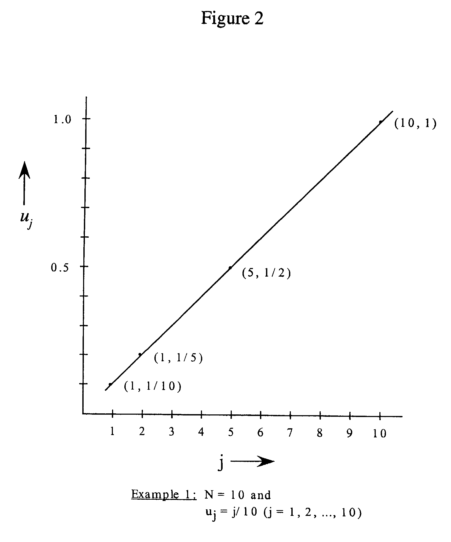
[0079]FIG. 2 shows an example of a one-dimensional linear signal u, expressible as vector of data u={uj}, where:
uj=j / N(j=1,2, . . . , N).
Then |∇u|j=1 for all j, as shown in FIG. 3. Note that |∇u| is a constant, independent of j. Thus, the compressed value of |∇u| is the same as the uncompressed value, as in FIG. 3. In this example, then, there is no error in the compressed and uncompressed values of |∇u|, nor is there any error in u or the reconstructed v.
[0080]In general, in this description the variable u will be used to refer to the original signal or data, and the variables v and w will be used to indicate the data after reconstruction (after of the first or second gradient or derivative, as will be discussed below).
[0081]Generally, lossy compression procedures will result in errors in signals u that do not comprise constant values, so earlier methods (which compress the signals u, and not the gradient of u as in the present invention) will lead to larger errors in the gradient ...
example 2
[0082]FIG. 4 shows an example one-dimensional signal, expressible as:
[0083]uj=j(j+1)2N2[0084](j=1,2, . . . , N)
Thus, for this signal |∇u|j=j / N, as shown in FIG. 5. (Note that the values of |∇u|j in Example 2 are the same as the values of uj in Example 1, which follows since the above function for uj in Example 2 was obtained by integrating the value uj=j / N from Example 1.)
[0085]If the approach of compressing the derivative (or gradient) of the function is used, rather than compressing the function itself, then we compute |∇|∇u∥, and obtain:
|∇|∇u∥j=1 for all j (as shown in FIG. 6).
[0086]The compression of this is error-free (for this example), and hence the errors in the reconstructed w (which approximates |∇u|) and v (which approximates u) are also zero, as is the error in the curvature approximating the curvature of z=u(x). Here,
[0087]k=uxx(1+ux2)32,
since there is no dependence on y. Thus, the method of FIG. 7 reduces the resulting error in this example.
[0088]Using the Laplacian ...
PUM
 Abstract
Description
Claims
Application Information