Stability determination method of non-linear active-disturbance-rejection control system

A technology of active disturbance rejection control and system stability, applied in the field of automation, can solve problems such as complex derivation process, complex system motion, and difficulty in popularization

Inactive Publication Date: 2015-12-16
PEOPLES LIBERATION ARMY ORDNANCE ENG COLLEGE +1
4 Cites 7 Cited by

AI-Extracted Technical Summary

Problems solved by technology

However, the introduction of nonlinear functions makes the system motion more complex, and the stability and performance analysis is more difficult. The stability analysis of nonlinear extended state observer and nonlinear active disturbance rejection control system has always been a difficult point.
[0003] Using the description function method to study the frequency domain stability of the active disturbance rejection control system with a single and two nonlinear links in the extended state observer, but due to the limited number of nonlinearities, the complexity of the g...

Abstract

The invention discloses a stability determination method of a non-linear active -disturbance-rejection control system. The method comprises steps of non-linear auto-disturbance-rejection control system establishment, system conversion, and stability determination of an indirect lurie system based on a robustness Popov criterion. The method has the following beneficial effects: the non-linear auto-disturbance-rejection control system is converted into an indirect lurie system and the system stability can be determined by using the robustness Popov criterion, and thus stability of a nominal system as well as robustness stability of the parameter shooting system can be determined, so that the operation becomes convenient; and the original complex non-linear extended state observer is changed into a variable-gain linear extended state observer and then stability is determined based on a routh criterion, so that the operation becomes simple and convenient.

Application Domain

Adaptive control

Technology Topic

System stabilityActive disturbance rejection control +1

Image

  • Stability determination method of non-linear active-disturbance-rejection control system
  • Stability determination method of non-linear active-disturbance-rejection control system
  • Stability determination method of non-linear active-disturbance-rejection control system

Examples

  • Experimental program(1)

Example Embodiment

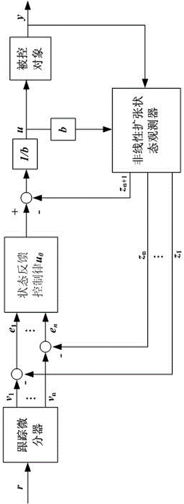
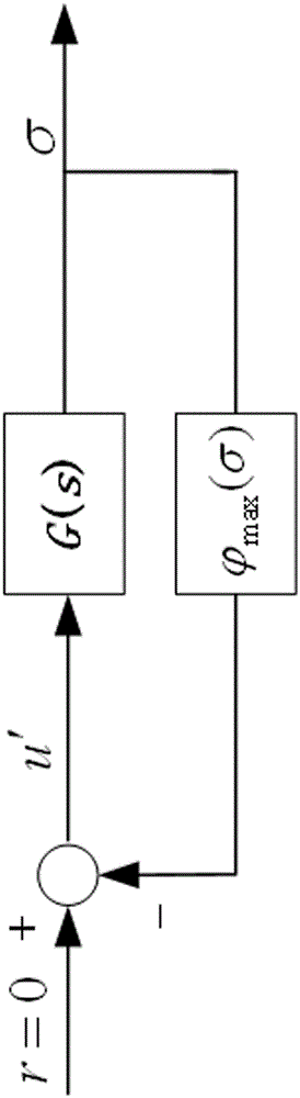
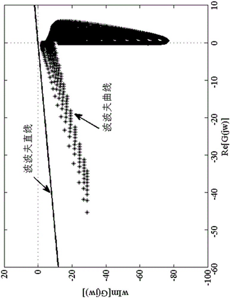
[0110] Combine below Figure 1-Figure 3 And the examples further illustrate the present invention.
[0111] Assuming that the input r of the tracking differentiator in A1 is 0, then the output v of the tracking differentiator is i (i=1, 2, ..., n) are all 0;
[0112] Taking the stability analysis of the second-order nonlinear auto disturbance rejection control system composed of the second-order controlled object and the nonlinear active disturbance rejection controller as an example, the application process of the present invention in practice is explained.
[0113] Stability analysis of nonlinear extended state observer based on Routh criterion.
[0114] Take a second-order linear constant controlled object as an example, its mathematical model is as follows:
[0115] x · 1 = x 2 x · 2 = - 3 x 1 - 5 x 2 + u y = x 1
[0116] (Eq. 29)
[0117] Where x 1 , X 2 Represents the state of the controlled object, Represents the first derivative of the corresponding state, y is the output of the controlled object, and the nonlinear error feedback control law u is the control input of the controlled object.
[0118] Design of nonlinear active disturbance rejection controller:
[0119] In view of the fact that the tracking differentiator is a relatively independent structure, it does not affect the stability of the system, and according to the output v of the tracking differentiator described in hypothesis A1 i (i=1, 2,..., n) are all 0, and no tracking differentiator is designed.
[0120] Since the controlled object is a second-order system, a typical third-order nonlinear extended state observer is designed as follows:
[0121] e = z 1 - y z · 1 = z 2 - β 01 · e z · 2 = z 3 - β 02 · f a l ( e , α 2 , δ ) + b u z · 3 = - β 03 · f a l ( e , α 3 , δ ) (Eq. 30)
[0122] The nonlinear error feedback control law u is designed as follows:
[0123] u=[k 1 fal(v 1 -z 1 , Α′ 1 ,Δ)+k 2 fal(v 2 -z 2 ,α′ 2 ,δ)-z 3 ]/b
[0124] (Eq. 31)
[0125] Here, the output v of the tracking differentiator described in hypothesis A1 i (i = 1, 2, ..., n) are all 0, then v 1 , V 2 All are zero.
[0126] Determine the parameters of the nonlinear active disturbance rejection controller: Let ω o =20, ω c = 10, β 01 =3ω 0 , k 2 = 2ω c , Δ=0.01, α 2 =0.5, α 3 =0.5,α' 1 =0.75,α' 2 = 1.5.
[0127] Stability analysis of nonlinear auto disturbance rejection control system based on robust Popov criterion:
[0128] According to (Equation 17) and (Equation 18), the forward channel transfer function expression of the second-order nonlinear active disturbance rejection control system is obtained:
[0129] G ( s ) = B ‾ 0 s 4 + B ‾ 1 s 3 + B ‾ 2 s 2 + B ‾ 3 s + B ‾ 4 A ~ 0 s 5 + A ~ 1 s 4 + A ~ 2 s 3 + A ~ 3 s 2 + A ~ 4 s + A ~ 5 (Eq. 32)
[0130] The coefficients of the numerator and denominator of (Equation 32) are as follows:
[0131] A ~ 0 = 1 , A ~ 1 = λ 2 , k 2 - a 1 , A ~ 2 = λ 1 k 1 - a 2 - a 1 λ 2 k 2
[0132] A ~ 3 = - a 1 λ 1 k 1 - a 2 λ 2 k 2 , A ~ 4 = - a 2 λ 1 k 1 , A ~ 5 = 0
[0133] B ~ 0 = λ ~ 01 β 01
[0134] B ~ 1 = λ ~ 02 β 02 - a 1 λ ~ 01 β 01 + λ ~ 01 β 01 λ 2 k 2
[0135] B ~ 2 = λ ~ 03 β 03 - a 1 λ ~ 02 β 02 - a 2 λ ~ 01 β 01 + λ ~ 01 β 01 λ 1 k 1 + λ ~ 02 β 02 λ 2 k 2 - a 1 λ ~ 01 β 01 λ 2 k 2
[0136] B ~ 3 = λ ~ 03 β 03 λ 2 k 2 - a 2 λ ~ 02 β 02 + λ ~ 02 β 02 λ 1 k 1 - a 2 λ ~ 01 β 01 λ 2 k 2
[0137] B ~ 4 = λ ~ 03 β 03 λ 1 k 1
[0138] Put ω o =20, ω c = 10, β 01 =3ω 0 , k 2 = 2ω c , Δ=0.01, α 2 =0.5, α 3 =0.5,α' 1 =0.75,α' 2 = 1.5, a 1 =-5, a 2 =-3, set
[0139] e i ∈[0,1](i=1, 2), e∈[0,1], substituting (Equation 32), we can get
[0140] A ~ 0 = 1 , A ~ 1 = [ 7 , 25 ] , A ~ 2 A [ 113 , 419 ] , A ~ 3 A [ 506 , 1640 ] , A ~ 4 A [ 300 , 949 ] , A ~ 05 = 0
[0141] B ~ 0 = A [ 6 , 60 ] , B ~ 1 A [ 282 , 1740 ] , B ~ 2 A [ 3.25 × 10 3 , 3.20 × 10 4 ] ,
[0142] B ~ 3 A [ 2.38 × 10 5 , 2.94 × 10 5 ] , B ~ 4 A [ 8.89 × 10 4 , 2.81 × 10 5 ]
[0143] The 16 transfer functions determined according to the robust Popov criterion are as follows,
[0144] G K = { G ( s ) : G ( s ) } = 60 s 4 + 282 s 3 + 3.25 X 10 3 s 2 + 2.94 X 10 5 s + 2.81 X 10 5 s 5 + 25 s 4 + 113 s 3 + 506 s 2 + 949 s , 60 s 4 + 1740 s 3 + 3.25 X 10 3 s 2 + 2.38 X 10 5 s + 2.81 X 10 5 s 5 + 25 s 4 + 113 s 3 + 506 s 2 + 949 s , 6 s 4 + 1740 s 3 + 3.20 X 10 4 s 2 + 2.38 X 10 5 s + 8.89 X 10 4 s 5 + 25 s 4 + 113 s 3 + 506 s 2 + 949 s , 6 s 4 + 282 s 3 + 3.20 X 10 4 s 2 + 2.94 X 10 5 s + 8.89 X 10 4 s 5 + 25 s 4 + 113 s 3 + 506 s 2 + 949 s , 60 s 4 + 1740 s 3 + 3.25 X 10 3 s 2 + 2.38 X 10 5 s + 2.81 X 10 5 s 5 + 25 s 4 + 419 s 3 + 506 s 2 + 300 s , 60 s 4 + 282 s 3 + 3.25 X 10 3 s 2 + 2.94 X 10 5 s + 2.81 X 10 5 s 5 + 25 s 4 + 419 s 3 + 506 s 2 + 300 s , 6 s 4 + 1740 s 3 + 3.20 X 10 4 s 2 + 2.38 X 10 5 s + 8.89 X 10 4 s 5 + 25 s 4 + 419 s 3 + 506 s 2 + 300 s , 6 s 4 + 282 s 3 + 3.20 X 10 4 s 2 + 2.94 X 10 5 s + 8.89 X 10 4 s 5 + 25 s 4 + 419 s 3 + 506 s 2 + 300 s ,
[0145] 6 s 4 + 1740 s 3 + 3.20 × 10 4 s 2 + 2.38 × 10 5 s + 8.89 × 10 4 s 5 + 7 s 4 + 419 s 3 + 1640 s 2 + 300 s , 60 s 4 + 282 s 3 + 3.25 × 10 3 s 2 + 2.94 × 10 5 s + 2.81 × 10 5 s 5 + 7 s 4 + 419 s 3 + 1640 s 2 + 300 s , 60 s 4 + 1740 s 3 + 3.25 × 10 3 s 2 + 2.38 × 10 5 s + 2.81 × 10 5 s 5 + 7 s 4 + 419 s 3 + 1640 s 2 + 300 s , 6 s 4 + 282 s 3 + 3.20 × 10 4 s 2 + 2.94 × 10 5 s + 8.89 × 10 4 s 5 + 7 s 4 + 419 s 3 + 1640 s 2 + 300 s , 6 s 4 + 282 s 3 + 3.20 X 10 4 s 2 + 2.94 X 10 5 s + 8.89 X 10 4 s 5 + 7 s 4 + 506 s 3 + 1640 s 2 + 949 s , 60 s 4 + 282 s 3 + 3.25 X 10 3 s 2 + 2.94 X 10 5 s + 2.81 X 10 5 s 5 + 7 s 4 + 506 s 3 + 1640 s 2 + 949 s , 60 s 4 + 1740 s 3 + 3.25 X 10 3 s 2 + 2.38 X 10 5 s + 2.81 X 10 5 s 5 + 7 s 4 + 506 s 3 + 1640 s 2 + 949 s , 6 s 4 + 1740 s 3 + 3.20 X 10 4 s 2 + 2.38 X 10 5 s + 8.89 × 10 4 s 5 + 7 s 4 + 506 s 3 + 1640 s 2 + 949 s }
[0146] (Eq. 33)
[0147] Then according to (Equation 33), the corresponding Popov curve is drawn as image 3 Shown. by image 3 It can be seen that all the Popov curves satisfy the Popov criterion, so the system is stable.
[0148] Stability analysis of nonlinear extended state observer based on Routh criterion:
[0149] Due to α 2 =α 3 , Therefore (Equation 28) is established, namely
[0150] β 01 β 02β 03 (Eq. 34)
[0151] Therefore, the nonlinear extended state observer represented by (Equation 30) is stable.
[0152] The above-mentioned embodiments are only preferred embodiments of the present invention, rather than exhaustive lists of possible embodiments of the present invention. For those of ordinary skill in the art, any obvious changes made to the present invention without departing from the principle and spirit of the present invention should be deemed to be included in the protection scope of the present invention.

PUM

no PUM

Description & Claims & Application Information

We can also present the details of the Description, Claims and Application information to help users get a comprehensive understanding of the technical details of the patent, such as background art, summary of invention, brief description of drawings, description of embodiments, and other original content. On the other hand, users can also determine the specific scope of protection of the technology through the list of claims; as well as understand the changes in the life cycle of the technology with the presentation of the patent timeline. Login to view more.
Why Eureka
Try Eureka