An image recognition method based on hierarchical feature extraction and multi-layer impulse neural network
A technology of spiking neural network and image recognition, applied in the field of spiking neural network, it can solve the problems of difficult feedback and discontinuous pulse delivery.
- Summary
- Abstract
- Description
- Claims
- Application Information
AI Technical Summary
Problems solved by technology
Method used
Image

Examples
Embodiment Construction
[0052] The present invention will be further described below in conjunction with the accompanying drawings.
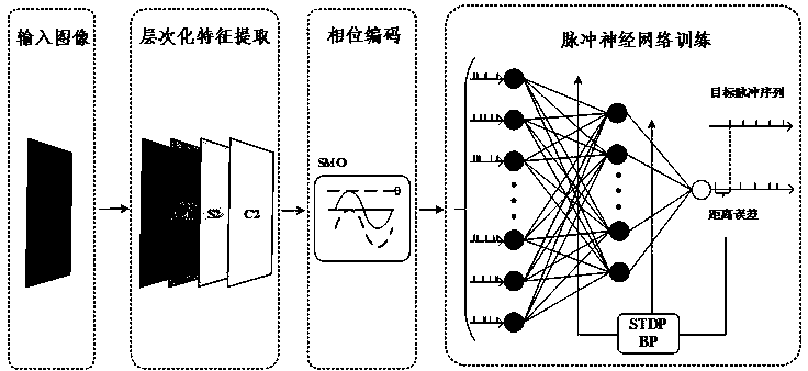
[0053] Figure 1 to Figure 4 Each stage of the entire image recognition process is shown separately. The process can be divided into 3 steps, and the specific content is as follows:
[0054] Step 1 Hierarchical Feature Extraction
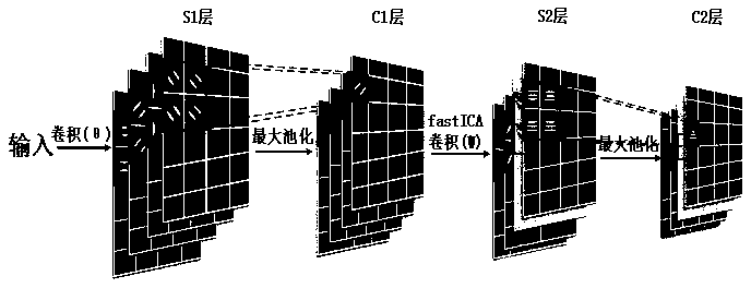
[0055] in figure 2 The overall process of hierarchical feature extraction is described. In this process, a four-layer model is adopted, which are S1 layer, C1 layer, S2 layer and C2 layer. The parameter values involved here are mainly for the MNIST data set. The specific operations of each layer are as follows:
[0056] 1.1S1 layer: extraction of edge information by Gabor filter
[0057] The cells in the primary visual cortex area are strongly sensitive to edge information, and the frequency and direction expression of the Gabor filter are considered to be similar to the human visual system, so in this step a two-dimensional Gabor fil...
PUM
 Abstract
Description
Claims
Application Information