[0015] The present invention will be further described below in conjunction with the accompanying drawings.
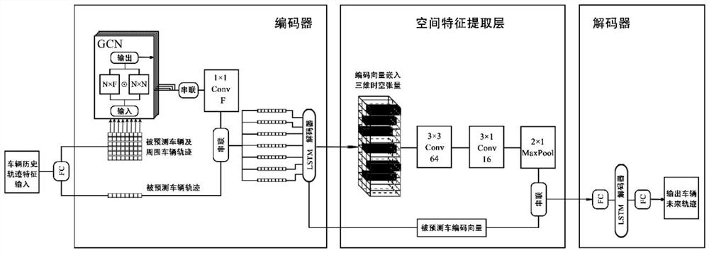
[0016] Step1: Model building
[0017] 1. Model input
[0018] The input feature value of trajectory prediction contains four necessary components, including the historical trajectory of the predicted vehicle, the historical trajectory of the vehicles around the predicted vehicle, the time TTC when the predicted vehicle and the surrounding vehicles reach the collision point, and the vehicle behavior at each moment.
[0019] (1) The historical trajectory of the predicted vehicle
[0020] The historical trajectory sequence of the predicted car can be expressed as:
[0021] X ego ={x (t-S) ,…,x (t-1) ,x (t) }
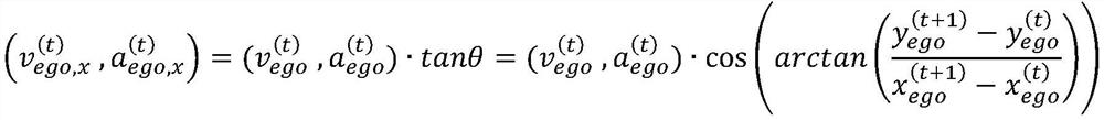
[0022] S is the length of the historical trajectory sequence, x (t) Represents the historical trajectory of the vehicle under test, t is the current moment, where:
[0023]
[0024] are the horizontal and vertical coordinates of the predicted car, is the horizontal and vertical speed of the predicted car, is the predicted lateral and longitudinal acceleration of the vehicle.
[0025] The calculation formulas of the predicted lateral and longitudinal vehicle speed and acceleration are as follows:
[0026]
[0027]
[0028] in is the vehicle speed and acceleration of the predicted vehicle driving direction, and θ is the heading angle of the vehicle when it is driving.
[0029] (2) Trajectories of vehicles around the predicted vehicle
[0030] Construct an occupancy grid map centered on the predicted vehicle, three lanes wide, multiple vehicle lengths and average head-to-head spacing, and define the vehicles contained in the occupied grid map as the surrounding vehicles of the predicted vehicle.
[0031] The vehicle trajectory sequence around the predicted car will be input to the convolution layer for feature extraction, so the number of vehicles around the predicted car is selected as a fixed value N, and the historical trajectory sequence of the predicted car neighbors is expressed as:
[0032]
[0033] (3) Collision time TTC
[0034] The collision time TTC between the predicted vehicle and surrounding vehicles, that is, the predicted vehicle and the j-th surrounding vehicle continue to travel according to the current driving direction and state to reach the meeting point The time, the coordinates of the encounter point are calculated by the horizontal and vertical coordinates of the vehicle that is predicted at the current moment and the horizontal and vertical coordinates of the neighbor vehicle j Calculation:
[0035]
[0036]
[0037] in, Indicates the heading angle of the predicted vehicle at time t, the heading angle of the jth neighbor vehicle Calculate using the horizontal and vertical vehicle speed at the current moment Then when the current speed of vehicle i is v i and maintain the heading angle θ i The time it takes to travel in the direction to the meeting point is:
[0038]
[0039] Then the difference between the time when the predicted vehicle and its neighbor vehicles arrive at the collision point, that is, the collision time TTC can be expressed as:
[0040] TTC=|t col,ego -t col,j |
[0041] t col,ego Represents the time when the vehicle under test reaches the collision point, t col,j Indicates the time when the neighbor vehicle reaches the collision point.
[0042] (4) Vehicle behavior
[0043] The vehicle behaviors on the road are divided into three types: lane keeping, left lane change, and right lane change.
[0044] Vehicle left/right lane change is defined as: record the sampling point lane at the current moment as L1, and the vehicle coordinates as (x (t) ,y (t) ). Traverse the sampling points of the historical data of the vehicle forward, and record the sampling point when the sampling point of the vehicle is pushed forward for the first time in the non-L1 lane as the lane change point, and the coordinates are (x c ,y c ). The coordinates of the third sampling point before changing the lane point are (x c+3 ,y c+3 ), the heading angle of the lane change point is calculated as:
[0045]
[0046] Let the angle between the coordinates of the vehicle at the sampling point and the coordinate of the lane change point be the minimum lane change judgment threshold:
[0047]
[0048] If the heading angles of the sampling points before and after the lane change point in the vehicle's historical trajectory satisfy the condition |θ cmin |≤|θ|≤|θ cmax|, then it is considered that the vehicle is changing lanes at this moment. When θ>0, it is a left lane change, and when θ<0, it is a right lane change. The sampling points that do not meet the conditions are marked as lane keeping behavior. Convert the judged vehicle behavior into the form of one-hot vector (for example, the one-hot vector form of lane keeping is: (0, 1, 0)), and use it as the input parameter of the model together with other conditions.
[0049] 2. Model structure
[0050] (1) Overall structure of the model
[0051] The overall structure of the model is as figure 1 As shown, the model consists of three large modules. Module 1 is the vehicle trajectory encoder module, which consists of a graph convolutional neural network layer and an LSTM encoder. The graph convolutional neural network layer is responsible for encoding the relationship between vehicles and the relationship characteristics of influence, and the LSTM encoder extracts the vehicle trajectory. The characteristics of the sequence in the time dimension. The second module is the spatial feature extraction layer, which consists of two convolutional layers and one pooling layer. Its function is to extract the spatial features formed by the vehicle position in the traffic scene. The third module is the decoder, namely the LSTM decoder, which uses the features extracted by the first two modules to output the predicted future vehicle trajectory coordinates through the decoder.
[0052] (2) Encoder module
[0053] Graph convolutional neural network layers:
[0054] A graph convolutional neural network is used to extract the relationship features of the non-Euclidean distance between the predicted car and surrounding vehicles. In the same traffic scene, the dimensional features (including coordinates, dynamic features, driver's intentions, etc.) among the moving vehicles are in a state of mutual influence. This state does not belong to a static space state that only relies on Euclidean distance to transmit, but a non-Euclidean graph structure connected to each other by virtual edges. The vehicle in the figure transmits its own feature information to the surrounding vehicles by connecting the edges, and also receives the feature information transmitted by the surrounding vehicles. Finally, the graph structure completes the transfer of the features, so that the features in the graph reach a new balance, that is, the feature update of the whole graph is completed. .
[0055] The number of nodes in the graph is N, the node feature is F, and the composition of the graph structure is expressed as G=(V, E). where V is the set of nodes, V ∈ R N , E is the edge set. The matrix formed by the connections between nodes in the graph is the adjacency matrix A, A∈R N×N. Since the relationship between the vehicles in the traffic scene is a dynamic relationship, it is impossible to directly define the edge connection between the vehicles. The present invention adopts the method of constructing an adaptive adjacency matrix, and expresses the adjacency matrix as:
[0056]
[0057] Among them, E 1 , E 2 ∈R N×F are two self-learning parameter matrices, E 1 Represents the output feature weight of the node, E 2 Represents the input feature weights of the node. will E 1 , E 2 The matrix after multiplying through the activation function ReLU and performing a row normalization is the most adjacency matrix that characterizes the spatial dependencies between nodes.
[0058] Then the feature update in each layer of network layer graph can be expressed as:
[0059] H l+1 =AH l W l
[0060] where W l Update the weight matrix of features for the lth graph convolutional layer. The network uses a total of k layers of graph convolution layers to extract node features, and finally the obtained k-layer features and the original features are concatenated to obtain k-order joint features:
[0061]
[0062] where || represents the concatenation symbol. The concatenated k-order features are passed through a convolutional layer with a convolution kernel size of 1×1 and an output channel of F to aggregate the feature information between each layer of the graph convolution, and the final output can represent all vehicles in the traffic scene. A graph feature context vector of non-Euclidean correlations.
[0063] LSTM encoder:
[0064] The LSTM encoder is used to obtain the temporal features of the vehicle feature sequence. The LSTM neuron contains three gated units: input gate, forget gate and output gate. The input gate controls the retention of hidden states and input features in neurons, and the forgetting gate controls the discarding of hidden states and input features. The input gate and the forgetting gate jointly construct new memory data c in the neuron, and the output gate Update the current neuron to pass the hidden state h and the output feature sequence output to the next neuron.
[0065] The input of the LSTM encoder is the graph feature context vector output by the graph convolutional neural network layer and the predicted vehicle trajectory sequence, and the output context vector can represent the hidden state of the entire input sequence at the last moment.
[0066] (3) Spatial feature extraction layer
[0067] Construct a 3D blank tensor with the same dimensions as the occupied raster image delimited by the surrounding vehicles selected by the predicted car frame and the context vector output by the encoder. The graph feature context vector of each vehicle output by the encoder is embedded into the corresponding grid in the grid graph to form a graph space-time tensor.
[0068] Aggregate and extract spatial features of tensors using convolution operations. First, the tensor is input into a convolutional layer with a convolution kernel of 3 × 3, and the number of input and output channels are both 64-dimensional. The function is to aggregate the spatial features inside each lane. The output tensor is then input to the convolution kernel with a size of 3×1 and the number of output channels is 16. Finally, the main feature information is extracted through a pooling layer with a pooling kernel size of 2×1 and a padding of (1,0), and finally the output tensor is dimensionally reduced to make it a one-dimensional vector. This vector is concatenated with the predicted car context vector as the feature tensor input to the decoder.
[0069] (4) LSTM decoder
[0070] The context vector output by the upper layer is expanded so that its time dimension is expanded to the same size as the time dimension of the predicted future trajectory. This sequence is fed into the LSTM encoder, which finally outputs the predicted trajectory.
[0071] Step2: Vehicle trajectory prediction
[0072] 1. Model training
[0073] (1) Training data
[0074] The model will use the historical trajectory features of the predicted car and the vehicles around the predicted car for 3s to predict the trajectory coordinates of the predicted car in the future 5s. The trajectory data of the vehicle is sampled at a certain frequency, and the historical trajectory data 3s before the current moment is merged with the current moment data to obtain a trajectory sequence composed of each sampling point as the input tensor of the model. Each sampling point contains 2 coordinates of the vehicle, 4 dynamic features, collision time TTC, and one-hot vector of vehicle behavior with length 3, a total of 10 eigenvalues. The coordinates of the predicted car are set as (0, 0), and the coordinates of the vehicles around the predicted car will be corrected to relative coordinates with the predicted car as the origin, which enhances the generalization and robustness of the model.
[0075] The width of the occupied grid map is three lanes centered on the prediction, that is, 3 grids, and the length is defined as 13 grids. The data form of the occupied grid map is a (3, 13) matrix, and the position of the predicted car in the occupied grid map is (2, 7). The vehicle data is embedded in the corresponding grid. If there is no vehicle in the grid, an all-zero vector with the same dimension as the vehicle data is embedded.
[0076] Integrate the acquired vehicle data into a training data set, take 128 sequences sampled each time and the sampling frequency is 5Hz as an example, the data size of the input encoder in the model is (128, 16, 40, 10) and (128, 16, 1, 10).
[0077] (2) Training environment
[0078] Use the pytorch framework to implement the training of the model, in which the model uses the Adam optimizer to accelerate the learning speed of the model, and the learning rate of the Adam optimizer is set to 0.001, so that the training can more accurately find the global optimal point. The loss function uses the root mean square error, RMSE, which visually calculates the dispersion between predicted and observed values.
[0079] The real vehicle data in the continuous time period in the trajectory prediction implementation scene is collected as the data set for model training, and the training set, validation set and test set used for model training are all taken from this data set. Use pytorch's built-in DateLoader module, use iterators to intelligently select data samples, and input data tensors in the corresponding format to the model.
[0080] (3) The training rounds are adjusted in real time according to the actual needs and training effects. After each round of training, a model parameter file is saved.
[0081] 2. Model running process
[0082] The parameters of each layer in the model are shown in Table 1. The data input layer is a fully connected layer with an input dimension of 10 and an output dimension of 32. The encoder consists of five layers of neural network. The first to third layers are graph convolution layers, and the input and output dimensions are 32; The channel is 32; the fifth layer is the LSTM encoder layer, the input dimension is 32, and the output dimension is 64. The spatial feature extraction module includes a three-layer neural network. The first layer is a convolutional layer with a convolution kernel size of (3×3) and both input and output channels are 64; the second layer is a convolution kernel with a size of (3×1) , the input channel is 64, the output channel is a convolutional layer of 16; the third layer is the maximum pooling layer, the pooling kernel size is (2×1), the upper and lower padding is 1, and the input and output channels are both 16. The decoder consists of three layers of neural network, the first layer is a fully connected layer, the input dimension is 227, and the output dimension is 128; the second layer is an LSTM decoder, and the input and output dimensions are both 128; the third layer is a fully connected layer, the input dimension is 128. The dimension is 32 and the output dimension is 2. The model works like figure 1 shown. The input parameters of the model go through the fully connected layer, and the feature dimension is expanded from 10 to 32.
[0083] (1) Encoder
[0084] The graph convolutional neural network layer contains 3 GCN layers, and the parameter matrix size of the adjacency matrix is (40, 10). Dropout is set in each layer, and the dropout ratio value is set to 0.2. The output feature dimension of each layer of the graph convolution layer remains the same as the initial dimension. After concatenation, the feature data with a length of 128 is obtained, and the feature length is changed to 32 through the convolution layer with a convolution kernel size of 1. Finally, the output value is passed through the activation function leakyReLU, and the negative slope is set to 0.2 to increase the nonlinearity of the network.
[0085] The input dimension of the LSTM encoder is 32, the output dimension is 64, and the number of layers is 1. Finally, the hidden state h of the last sampling time is output as an encoding vector, which is passed to the next module after passing through the activation function leakyReLU.
[0086] (2) Spatial state extraction layer
[0087]The encoding vector of each vehicle is embedded in the corresponding occupied grid map tensor. If the nearby vehicle and the predicted vehicle exist in the same grid, the encoding vectors of the two are added together. The spatial tensor is input into the pooling layer with the pooling kernel (2×1) and the padding (1,0) after passing through the convolutional layers with the convolution kernels of (3×3) and (3×1). The spatial feature map composed of the historical trajectory points of the predicted vehicle and the surrounding vehicles is extracted, and the size is (5×1). Finally, all vehicle features contained in the output feature map are fused into a one-dimensional vector through dimensionality reduction processing, and the vector and the predicted vehicle encoding vector are passed to the decoder module in series.
[0088] (3) Decoder
[0089] The input data is passed through a fully connected layer to change the feature dimension to the input dimension 128 of the LSTM decoder. Each feature vector in the data sample collects the time, space, and graph feature information of the sequence, and the feature vector is copied to expand the time dimension to the length of the predicted time series. After the data passes through the encoder, it passes through a fully connected layer, and outputs the vehicle trajectory coordinate sequence of the predicted vehicle 5s in the future at the current moment to complete the trajectory prediction task.
[0090] Table 1
[0091]
[0092]
[0093] The series of detailed descriptions listed above are only specific descriptions for the feasible embodiments of the present invention, and they are not used to limit the protection scope of the present invention. All should be included within the protection scope of the present invention.