

Motor imagery classification method based on optimal narrow band feature fusion
A technology of motor imagery and feature fusion, applied in neural learning methods, complex mathematical operations, and pattern recognition in signals, etc., can solve problems such as difficulty in obtaining satisfactory results, affecting classification performance, and losing potential information.
- Summary
- Abstract
- Description
- Claims
- Application Information
AI Technical Summary
Problems solved by technology
Method used
Image

Examples
Embodiment Construction
[0065] In order to make the purpose, technical solution and key points of the present invention clearer, the following will further describe in detail the embodiments of the present invention in conjunction with the accompanying drawings.
[0066] A motor imagery classification method based on optimal narrow-band feature fusion, comprising the following steps:
[0067] Step 1: Obtain motor imagery EEG signals
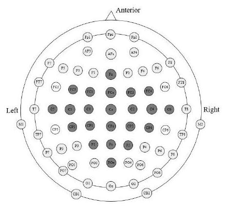
[0068] The experiment selects the BCI competition IV 2a four-category motor imagery dataset (hereinafter collectively referred to as the BCI competition dataset). It includes four types of motor imagery tasks: left hand, right hand, feet and tongue. It includes EEG signals from 22 electrodes and EOG signals from 3 electrodes. The signal sampling rate is 250Hz and processed by 0.5-100Hz band-pass filtering. .
[0069] Step 1.1: In the BCI competition data set, 9 subjects performed four types of motor imagery tasks, and a total of two experiments were conducted. Each e...
PUM
 Abstract
Description
Claims
Application Information