Apparatus and method for imaging a subsurface using frequency-domain elastic reverse-time migration

Active Publication Date: 2012-03-01
SEOUL NAT UNIV R&DB FOUND
25 Cites 17 Cited by

AI-Extracted Technical Summary

Problems solved by technology

However, since elastic medium has all of P, S and Rayleigh waves, it is not easy to obtain a location for imaging since undesired artifacts may be produced due to a correlation between the P, S and Rayleigh waves.
However, s...

Benefits of technology

[0015]Therefore, according to the subsurface imaging technique using frequency-domain elastic reverse-time migration, by applying Helmholtz decomposition to the frequency domain for division into P- and S-wave potentials, a complex topographical ...

Abstract

Provided are an apparatus and method for imaging a subsurface using frequency-domain reverse-time migration in elastic medium. The subsurface imaging method represents a frequency-domain imaging condition as convolution of measured data and a partial derivative wavefield. That is, the subsurface imaging method applies a back-propagation algorithm to represent an imaging condition as convolution of a virtual source and a back-propagated wavefield. Then, the subsurface imaging method divides a virtual source vector and the back-propagated wavefield represented by a displacement vector into P- and S-wave potentials through Helmholtz decomposition, thereby providing a new imaging condition.

Application Domain

Technology Topic

Image

  • Apparatus and method for imaging a subsurface using frequency-domain elastic reverse-time migration
  • Apparatus and method for imaging a subsurface using frequency-domain elastic reverse-time migration
  • Apparatus and method for imaging a subsurface using frequency-domain elastic reverse-time migration

Examples

  • Experimental program(1)

Example

[0020]Throughout the drawings and the detailed description, unless otherwise described, the same drawing reference numerals will be understood to refer to the same elements, features, and structures. The relative size and depiction of these elements may be exaggerated for clarity, illustration, and convenience.
DETAILED DESCRIPTION
[0021]The following description is provided to assist the reader in gaining a comprehensive understanding of the methods, apparatuses, and/or systems described herein. Accordingly, various changes, modifications, and equivalents of the methods, apparatuses, and/or systems described herein will be suggested to those of ordinary skill in the art. Also, descriptions of well-known functions and constructions may be omitted for increased clarity and conciseness.
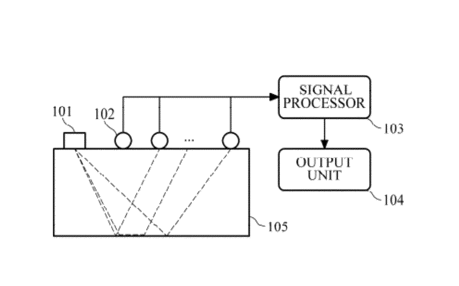
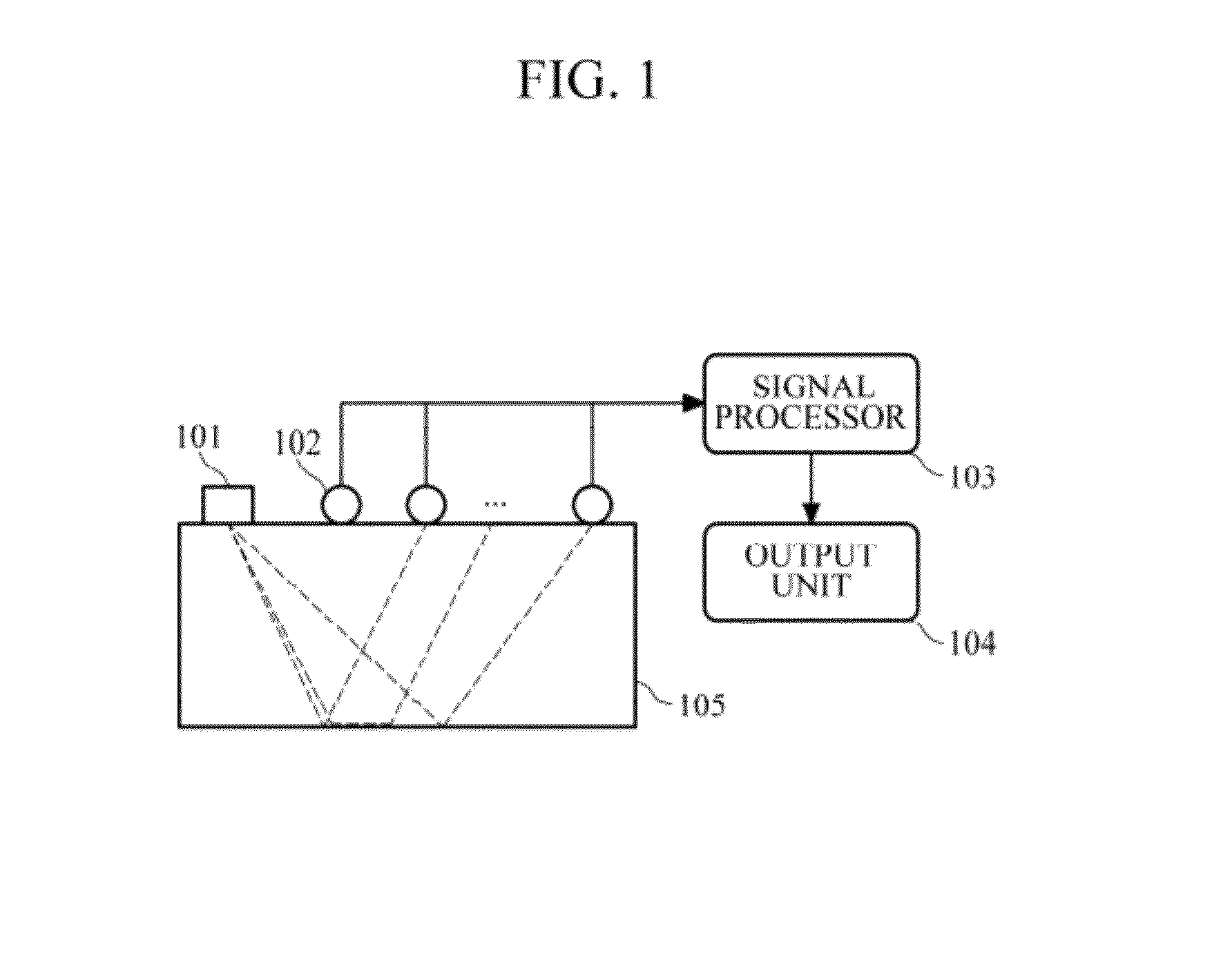
[0022]FIG. 1 is a diagram illustrating an example of a subsurface imaging apparatus using frequency-domain reverse-time migration in elastic medium. Referring to FIG. 1, the subsurface imaging apparatus may include a source 101, a receiver 102, a signal processor 103, and an output unit 104.
[0023]The source 101 is used to generate waves (source wavelets) toward a region 105 to be observed. The kind of the source 101 is not limited, and may be a dynamite, an electric vibrator, etc. The source 101 may use well-known waves or arbitrary waves generated by a specific apparatus. For example, surface exploration generally uses waves generated by vibroseis, without knowing accurate information about the waveforms of used sources. In this case, it is needed to estimate sources when obtaining reverse-time migration images.
[0024]The receiver 102 detects seismic signals propagated from the region 105 to be observed, and the kind of the receiver 102 is also not limited. For example, the receiver 102 may be a seismic detector, or the like. For efficient detection of seismic, a plurality of receivers 102 may be disposed in a predetermined pattern (for example, in a lattice pattern) on or around the region 105. The output unit 104 is used to output signals (for example, migrated images) received from the signal processor 103, and may be a display that outputs images or graphic data.
[0025]The signal processor 103 may be a signal processor or a computer program to generate a migration images showing the subsurface of the region 105 using a virtual source vector and the seismic data (the measured data) received from the receiver 102. The source vector may be estimated using the received seismic data by the signal processor 103 based on predetermined model conditions, and a method of estimating the source wavelet is not limited. The migration image signal generated by the signal processor 103 is transferred to the output unit 104 and then output. The signal processor 103 may use the measured data and the virtual source vector to generate a migrated image with respect to P- and/or S-wave, representing the subsurface of the region 105, using conditions for imaging seismic, which will be described later.
[0026]According to the current example, the signal processor 103 processes signals in the frequency domain, not in the time domain. For example, the signal processor 103 transforms equation representing a migrated image in the time domain to equation representing a migrated image in the frequency domain, and then applies Helmholtz decomposition to horizontal and vertical displacements of seismic to divide into the P- and S-wave potentials, in consideration of the fact that virtual source signals and back-propagated waves all contain P, S and Rayleigh waves in elastic medium. Hereinafter, signal processing by the signal processor 103 will be described in more detail.
Imaging Conditions for Acoustic Waves
[0027]A migration image with respect to arbitrary model parameters in the time domain may be expressed as equation 1, below. According to equation 1, an imaging condition in the time domain is expressed as a zero-lag cross-correlation between an arbitrary parameter wavefield and measured data on receivers in the time domain.
φ k = ∫ [ ∂ u ( t ) ∂ p k ] T ( t ) t , ( 1 )
where φk denotes the migration image for the k-th model parameter, pk denotes the k-th model parameter, T denotes the prefix of the matrix, and u(t) and d(t) denote the frequency-domain modeled wavefield and the measured wavefield, respectively. By transforming equation 1 to equation in the frequency domain, the reverse-time migration image can be expressed by convolution of the conjugate of the real measured data with the partial derivative wavefield. The migration image may be induced as:
φ k = ∫ Re { [ ∂ u ~ ∂ p k ] T d ~ * } ω , ( 2 )
where ω is the angular frequency, the superscript * denotes the complex conjugate, and ũ and {tilde over (d)} are the frequency-domain modeled wavefield and the measured wavefield, respectively. Meanwhile, it has been well-known that a frequency-domain wave equation can generally be expressed as a matrix like equation 3, below.
Sũ={tilde over (f)}  (3)
where S is the complex impedance matrix, and {tilde over (f)} is the frequency-domain source vector. By taking the partial derivative of both sides of equation 3 with respect to the k-th model parameter, equation 4 can be obtained as:
S ∂ u ~ ∂ p k = - ∂ S ∂ p k u ~ or ∂ u ~ ∂ p k = S - 1 v k , where v k ( v k = - ∂ S ∂ p k u ~ ) ( 4 )
is the k-th virtual source vector, and S−1 is the inverse matrix of the complex impedance matrix.
[0028]By putting equation 4 into equation 4, equation 4 can be rewritten to equation 5 below:
φk=∫{(vk)TS−1{tilde over (d)}}dω (5)
[0029]It can be seen from equation 5 that an imaging condition for acoustic medium can be defined in the frequency domain by convolving the virtual source vector with a wavefield S−1{tilde over (d)} obtained by back-propagating the measured data.
Imaging Conditions for Elastic Waves
[0030]2-D seismic wave equation can be defined as equations 6 and 7 below:
ρ ∂ u ∂ t 2 = ∂ σ xx ∂ x + ∂ σ xz ∂ z and ( 6 ) ρ ∂ v ∂ t 2 = ∂ σ zx ∂ x + ∂ σ zz ∂ z , ( 7 )
where u and v denote horizontal and vertical displacements, respectively, and σxx, σxz, σzz denote stresses in the xx, xz, and zz directions, respectively.
[0031]The stress equations in the xx, xz, and zz directions can be defined as equations 8, 9, and 10, respectively.
σ xx = ( λ + 2 μ ) ɛ xx + λɛ zz = ( λ + 2 μ ) ∂ u ∂ x + λ ∂ v ∂ z , ( 8 ) σ xz = μ ɛ xz = μ ( ∂ v ∂ x + ∂ u ∂ z ) = μ ɛ zx = σ zx , and ( 9 ) σ zz = λ ɛ xx + ( λ + 2 μ ) ɛ zz = λ ∂ u ∂ x + ( λ + 2 μ ) ∂ v ∂ z ( 10 )
where ρ is the density of medium, λ and μ are the Lame's constants, u and v are the horizontal and vertical displacements, respectively, εxx, εxz, and εzz are strains in the xx, xz, and zz directions, and σxx, σxz, σzz are stresses in the xx, xz, and zz directions, respectively.
[0032]By putting the stress equations defined by equations 8, 9, and 10 into equations 6 and 7 and then performing Fourier transformation, equations 11 and 12 are deduced.
- ρ ω 2 u ~ - ∂ ∂ x { ( λ + 2 μ ) ∂ u ~ ∂ x + λ ∂ v ~ ∂ z } - ∂ ∂ z { μ ( ∂ v ~ ∂ x + ∂ u ~ ∂ z ) } = 0 , and ( 11 ) - ρω 2 v ~ - ∂ ∂ x { μ ( ∂ v ~ ∂ x + λ ∂ u ~ ∂ z ) } - ∂ ∂ z { λ ∂ u ~ ∂ x + ( λ + 2 μ ) ∂ v ~ ∂ z } = 0 , ( 12 )
where ũ and {tilde over (v)} denotes horizontal and vertical displacements in the frequency domain, respectively.
[0033]Meanwhile, modeling of seismic wave equation in the frequency domain also can be expressed, like acoustic wave equation, as a matrix such as equation 13.
Seue=fe,   (13)
where Se represents the complex impedance matrix of seismic wave equation, ũe is the horizontal and vertical displacement vector in the frequency domain, and {tilde over (f)}e is the horizontal and vertical source vector in the frequency domain.
[0034]Since modeling of seismic wave equation in the frequency domain can be expressed as a matrix like equation 13, a reverse-time migration image in elastic medium can be represented as equation 14.
φ k = ∫ Re ( ( v ke ) T S - 1 d ~ e * } ω , where v ke ( v ke = - ∂ S e ∂ p k u ~ e ) ( 14 )
is the virtual source vector in elastic medium, and {tilde over (d)}e is the horizontal and vertical displacement vector measured in elastic medium.
[0035]It can be seen from equation 14 that a reverse-time migration image in elastic medium can be represented as convolution of the vertical source vector with the back-propagated wavefield, like equation 5 (reverse-time migration image in acoustic medium). However, unlike acoustic medium, in elastic medium, both the vertical source vector and the back-propagated wavefield contain all of P, S, and Rayleigh waves. When convolution is performed on seismic waves into which various kinds of waves are mixed, undesired artifacts may be generated, and as a result, it is difficult to obtain a clean subsurface image.
[0036]In 1990, Dellinger and Etgen suggested a method of dividing the seismic horizontal and vertical displacements into P- and S-wave potentials using divergence (∇•) and curl (∇x) operators. Thereafter, in 2008, Yan and Sava applied the method to the time domain to divide a seismic displacement vector into the potential of each displacement. According to Yan and Sava, an imaging condition in the time domain can be expressed as equation 15, below:
Iij(x)=∫asi(x,t)ari(x,t)dt (15)
where ai and aj denote the divided P- and S-wave potentials. According to equation 15, four migration images of Ipp, Ips, Isp, and Iss can be obtained.
[0037]According to an example, based on the fact that an imaging condition in the frequency domain is represented as convolution of a virtual source vector with a wavefield obtained by back-propagating measured data, by applying the divergence and curl operators to the virtual source vector and the back-propagated wavefield displacement vector, imaging conditions similar to Ipp and Iss obtained from equation 15 are induced, which can be written as equations 16 and 17, below.
(φk)PP=∫Re{∇·[(vke)T]∇·[Se−1{tilde over (d)}e*]}dω (16)
(φk)SS=∫Re{∇x[(vke)T]∇x[Se−1{tilde over (d)}e*]}dω (17)
Model Parameters
[0038]The current example considers the fact that elastic medium, unlike acoustic medium, includes various model parameters. A migration image in elastic medium may depend on various model parameters. Upon actual migration, a virtual source vector in elastic medium may be obtained by differentiating a complex impedance matrix with respect to individual model parameters. A complex impedance matrix that is used upon modeling of a seismic wave equation is composed of the Lame's constant and density. However, the subsurface imaging method according to the current example uses P- and S-wave velocities as interested model parameters. Like the Mora's method (1987), the subsurface imaging method according to the current example may use a chain rule to generate a virtual source vector.
[0039]A correlation between P- and S-waves, the Lame's constant, and density can be represented as equations 18 and 19, below.
λ=ρVp2−2ρVs2 (18)
μ=ρVs2 (19)
[0040]Derivatives of complex impedance for the P- and S-wave velocities can be defined using equations 18 and 19 and the chain rule, as follows. Accordingly, virtual source vectors for the P- and S-wave velocities can be defined as equations 20 and 21.
( v ke ) p = - ∂ S e ∂ v p u ~ e , and ( 20 ) ( v ke ) s = - ∂ S e ∂ v s u ~ e , where ∂ S e ∂ v p = 2 ρ v p ∂ S e ∂ λ , and ∂ S e ∂ v s = - 4 ρ v s ∂ S e ∂ λ + 2 ρ v s ∂ S e ∂ μ . ( 21 )
Scaling
[0041]In a general migration condition for acoustic medium, a migration image is scaled with an autocorrelation of a modeled wavefield at a source location, so that the amplitude of the migration image is corrected.
[0042]As described above, the virtual source vector used in the current example means a modeled wavefield at a source location in the general migration condition. Therefore, according to the current example, a pseudo-Hessian matrix is created like the conventional method, and the migration image may be scaled using the diagonal of the pseudo-Hessian matrix.
[0043]Also, normalization may be performed such that migration images obtained for individual frequencies have the same weight, and then the normalized image is again normalized, thereby obtaining a final migration image. The final migration image is represented with is respect to P- and S-waves as equations 22 and 23, which are called a PP method and a SS method.
( φ k ) pp = NRM [ ∫ NRM [ Re { ∇ · [ ( v ke ) T ] ∇ · [ S e - 1 d ~ e * ] } Re { diag [ ( ∇ · [ ( v ke ) T ] ) T ( ∇ · [ ( v ke ) T ] ) ] + λ I } ] ω ] ( 22 ) ( φ k ) ss = NRM [ ∫ NRM [ Re { ∇ × [ ( v ke ) T ] ∇ × [ S e - 1 d ~ e * ] } Re { diag [ ( ∇ × [ ( v ke ) T ] ) T ( ∇ × [ ( v ke ) T ] ) ] + λ I } ] ω ] ( 23 )
Simulation (Marmousi-2 Model)
[0044]In order to verify the reverse-time migration in elastic medium, the Marmousi-2 model was used to perform simulation. For imitating the accurate earth state, new P- and S-wave velocity models and a density model were designed by eliminating a water layer from the conventional Marmousi-2 model.
[0045]In order to create observed data about the Marmousi-2 model from which the water layer has been eliminated, the time-domain 2D cell-based FDM modeling algorithm has been used. In this case, vertical sources were placed at regular intervals of 20 m on the earth surface, and horizontal and vertical displacements have been measured on 1,101 receivers located at regular intervals of 10 m. The total measurement time was 6 seconds. Also, since the S-wave velocity of the Marmousi-2 velocity model had a region with a very low speed, a first-order derivative Gaussian function whose maximum frequency was 5 Hz has been used as a transmission waveform. In the simulation, migration images with respect to the P- and S-waves have been obtained using the conventional method and the P- and S-wave imaging methods according to the above-described examples, based on a slightly smoothed velocity model.
[0046]FIGS. 2A, 2B, and 2C show P-wave migration images obtained by the conventional method, by the PP method (see equation 22), and by the SS method (see equation 23), respectively.
[0047]FIGS. 3A, 3B, and 3C show S-wave migration images obtained by the conventional method, by the PP method, and by the SS method, respectively. It can be seen from FIGS. 2A, 2B, 2C, 3A, 3B, and 3C that the migrated images obtained by the PP and SS methods provide more detailed information about a subsurface than the migration image obtained by the conventional method.
[0048]A number of examples have been described above. Nevertheless, it will be understood that various modifications may be made. For example, suitable results may be achieved if the described techniques are performed in a different order and/or if components in a described system, architecture, device, or circuit are combined in a different manner and/or replaced or supplemented by other components or their equivalents. Accordingly, other implementations are within the scope of the following claims.

PUM

no PUM

Description & Claims & Application Information

We can also present the details of the Description, Claims and Application information to help users get a comprehensive understanding of the technical details of the patent, such as background art, summary of invention, brief description of drawings, description of embodiments, and other original content. On the other hand, users can also determine the specific scope of protection of the technology through the list of claims; as well as understand the changes in the life cycle of the technology with the presentation of the patent timeline. Login to view more.

Similar technology patents

Classification and recommendation of technical efficacy words

  • Efficiently compute

Traffic data management and simulation system

ActiveUS7155376B2Low granularityEfficiently computeData processing applicationsDetection of traffic movementTraffic simulatorTraffic analysis
Owner:CALIPER CORPORATION

Methods for determining block averages for film grain simulation

ActiveUS20060083316A1Efficiently computeLow memory bandwidth requirementTelevision system detailsImage enhancementFilm grainMemory bandwidth
Owner:INTERDIGITAL CE PATENT HLDG
Why Eureka
Try Eureka