Information processing device, information processing system, information processing method, storage medium and program

[0034] Hereinafter, an embodiment of the present invention will be described with reference to the drawings. In addition, in the drawings, the same constituent elements are labeled as the same reference numerals, and the description will be omitted.

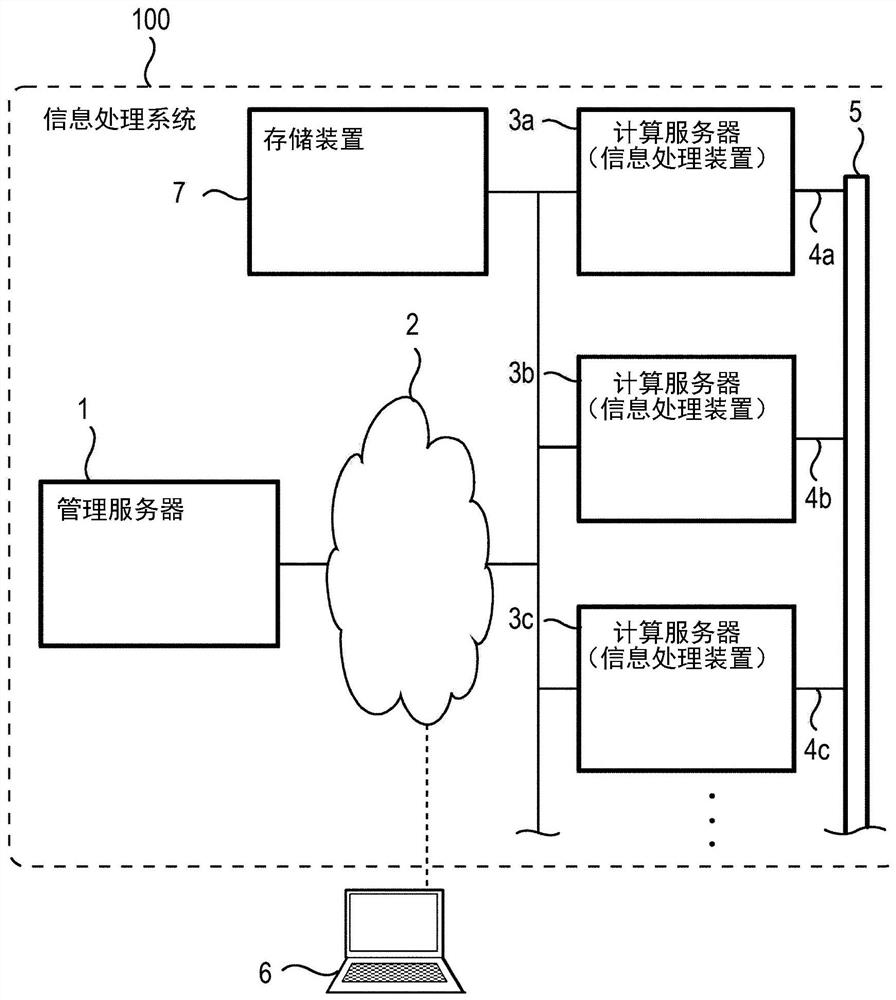
[0035] figure 1 It is a block diagram showing the configuration example of the information processing system 100. figure 1 The information processing system 100 is provided with management server 1, network 2, computing server (information processing apparatus) 3a to 3c, cables 4a to 4c, switch 5, and storage device 7. In addition, figure 1 A client terminal 6 that can communicate with the information processing system 100 is shown in the information processing system 100. Manage Server 1, computing servers 3a to 3c, the client terminal 6, and storage device 7 can communicate with each other via network 2. For example, the calculation servers 3a to 3c can store data in the storage device 7, or read data from the storage device 7. Network 2, for example, multiple computer networks being connected to each other. Network 2 can use wired, wireless, or a combination thereof as a communication medium. Further, as an example of the communication protocol used in the network 2, there is TCP / IP, but the type of the communication protocol is not particularly limited.

[0036] Further, the calculation servers 3a to 3c are connected to the switch 5 via cables 4a to 4c, respectively. Cables 4a to 4c and switch 5 form an interconnection between the calculation server. Calculation servers 3a to 3c can also communicate with each other via this interconnection. The switch 5 is, for example, a switch of InfiniBand (unlimited bandwidth). Cables 4a to 4c are, for example, INFINIBAND cables. However, you can also use the switch / cable of the wired LAN instead of InfiniBand's switch / cable. Regarding the communication standards and communication protocols used in cables 4a to 4c and switch 5, it is not particularly limited. As an example of the client terminal 6, you can list a notebook PC, a desktop PC, a smartphone, a tablet, a vehicle terminal, and the like.

[0037] In the solution of the combination optimization problem, it is possible to perform parallellation and / or dispersion of processing. Therefore, the processor of the calculation servers 3a to 3c and / or the calculation servers 3a to 3c can be allocated to perform the steps of performing a part of the calculation process, or may perform the same calculation processing in parallel with different variables. The management server 1 will change, for example, the combination of the user input into the form of each computing server can handle, and control the computing server. Further, the management server 1 obtains the calculation result from each computing server, and the summary calculation result is converted into a solution of the combined optimization problem. Thus, the user can obtain the solution of the combination optimization problem. Set to a combination optimization problem to unpack the optimal solution and analog solution to the optimal solution.

[0038] exist figure 1 Three computing servers are shown in it. However, the number of tables of the computing server included in the information processing system is not limited. In addition, there is no particular limitation on the calculation server used in the solution optimization problem in combination. For example, the computing server contained in the information processing system can also be 1 set. Additionally, a solution of combined optimization problems can be performed using any of the plurality of computing servers included in the information processing system. In addition, hundreds of computing servers can be included in the information processing system. The compute server can be servers set in the data center, or a desktop PC disposed in the office. In addition, the computing server can also be a plurality of types of types set in different locations. There is not particularly limited regarding the type of information processing apparatus used as a computing server. For example, the computing server can either a general purpose computer or a dedicated electronic circuit or a combination thereof.

[0039] figure 2 It is a block diagram showing the configuration example of the management server 1. figure 2 The management server 1 is, for example, a computer including a central arithmetic processing device (CPU) and a memory. The management server 1 is provided with processor 10, the storage unit 14, the communication circuit 15, the input circuit 16, and the output circuit 17. Set to processor 10, the storage unit 14, the communication circuit 15, the input circuit 16, and the output circuit 17 are connected to each other via the bus 20. The processor 10 includes a management unit 11, a conversion unit 12, and a control unit 13 as an internal constituent element.

[0040]The processor 10 is performing an operation, an electronic circuit for controlling the management server 1. The processor 10 is an example of a processing circuit. As the processor 10, for example, using the CPU, microprocessor, ASIC, FPGA, PLD, or a combination thereof. Management unit 11 provides an interface 6 for terminal operation management server 1 via the user client. Examples of the management section 11 provides an interface may include API, CLI, web pages. For example, a user may input information to optimize problem management unit 11 via the combination, or view and / or download the solution of the optimization problem computed combination. 12 combinatorial optimization conversion calculation unit for the transform of the server can handle. The control unit 13 transmits a control command to each compute server. The control unit 13 from the calculation result obtained in the calculation of each server, a plurality of conversion calculation unit 12 summarizes the results converted to a combination of solutions of the optimization problem. Further, the control unit 13 may specify the contents of each calculation process executed by a processor or server within each server.

[0041] Storage unit 14 stores a program management server 1 executes the program and data required for the data generated by the program, including a variety of data. Here, the program is set to include both OS and applications. The storage unit 14 may be a volatile memory, nonvolatile memory, or a combination thereof. Examples of volatile memory, there are DRAM, SRAM and the like. As examples of nonvolatile memory include NAND flash, NOR flash, ReR AM or MRAM. Further, as the storage unit 14 may be a hard disk, optical disk, magnetic tape, or an external storage device.

[0042] The communication circuit 15 transmits and receives data between the respective devices connected to the network 2. The communication circuit 15, for example, wired LAN NIC (Network Interface Card, a network interface card). However, the communication circuit 15 may be other types of wireless LAN communications circuitry. An input circuit 16 for input to the data management server 1. The input circuit 16 includes a set e.g. USB, PCI-Express or the like as the external port. exist figure 2 Example, the operating device 16 is connected to the input circuit 18. Operating means 18 is used to input information to the management server device 1. Operation means 18 such as a keyboard, mouse, touch pad, voice recognition apparatus and the like, but is not limited thereto. The output circuit 17 implemented data output from the management server 1. The output circuit 17 includes a set HDMI, DisplayPort or the like as the external port. exist figure 2 Example, the display device 19 and the output circuit 17 is connected. Examples of the display device 19, with a LCD (Liquid Crystal Display), organic EL (organic electroluminescence) display, or a projector, but is not limited thereto.

[0043] 1 management server administrator can use the operation device 18 and a display device 19 for maintenance management server 1. Further, the operating device 18 and display device 19 may be combined into a management server. Further, on the management server 1 may not necessarily connected to the operating device 18 and a display device 19. For example, the manager may be capable of maintenance management server 2 and the information terminal 1 is a communication network.

[0044] image 3 Shows an example of the data management server 14 stored in the storage unit 1. exist image 3 The storage unit 14, stores issue data 14A, 14B calculation data, management procedures. 14C, 14D and the control program conversion program 14E. For example, the problem of data comprising data 14A combinatorial optimization problem. For example, computing data collected from 14B comprise respective calculation results to the server. For example, the management program 14C is a program management unit 11 implement the functions of the above-described. For example, the conversion program 14D is a program to realize the functions of the conversion section 12. For example, the control program 14E is a program to realize the above-described functions of the control unit 13.

[0045] Figure 4 It is a block configuration example of the compute servers. Figure 4 Compute servers, for example, alone or shared with other server information calculation processing means calculates a first vector and second vector execution.

[0046] Figure 4 An exemplary calculation showing the structure of the server 3a. Other servers can be either calculated with the computing server 3a same structure, or may be calculated with a different configuration server 3a.

[0047] 3a calculation server includes a communication circuit 31, for example, a shared memory 32, the processor 33A ~ 33D, the memory 34, the host bus adapter 35. The communication circuit 31, a shared memory 32, the processor 33A to 33D, the memory 34 and the host bus adapter 35 connected to one another via a bus 36.

[0048] The communication circuit 31 transmits and receives data between the respective devices connected to the network 2. The communication circuit 31, for example, wired LAN NIC (Network Interface Card: a network interface card). However, the communication circuit 31 may be other types of wireless LAN communications circuitry. Shared memory 32 is a memory from the processor can be accessed 33A ~ 33D. Examples of shared memory 32 may include DRAM, SRAM and other volatile memory. However, as the shared memory 32 may be other kinds of memory using nonvolatile memory. Shared memory 32 may be configured, for example, for the storage elements as the first vector and the second vector. 33A ~ 33D processor capable of sharing data via the shared memory 32. Further, the calculation may not necessarily be all of the memory of the server 3a as a shared memory configuration. For example, the memory may be part of the computing server 3a is configured to only be able to access the local memory from a processor. Further, the shared memory 32 and the memory 34 described later is an example of a storage unit of the information processing apparatus.

[0049] The processor 33A ~ 33D is to perform calculation processing of the electronic circuit. The processor may be, for example, CPU (CentralProcessing Unit: central processing unit), GPU (Graphics Processing Unit: Graphics Processing Unit), FPGA (Field-Programmable Gate Array: a field programmable gate array) or an ASIC (Application SpecificIntegrated Circuit: ASIC any) and it may also be a combination thereof. In addition, the processor may be a CPU core or CPU threads. In the case where the processor is a CPU, calculated on the number of slots provided in the server 3a is not particularly limited. Further, the processor may be connected to other components of the computing server 3a via PCI express bus or the like.

[0050] exist Figure 4 Example, the calculation server is provided with four processors. However, the processor calculates the number of servers included in a stage may be different from this. For example, the number calculated by the processor of the server installation and / or species may be different. Here, the processor is an example of a processing circuit of the information processing apparatus. The information processing apparatus may be provided with a plurality of processing circuits.

[0051] The information processing apparatus is configured, for example, repeatedly updating the first variable x i (I = 1,2, ..., N) is the first vector and a second element of the first variable corresponding to the variable y i (I = 1,2, ..., N) for the second vector element.

[0052] For example, the information processing apparatus is a processing circuit may be configured to update the first vector by a second variable weighted and added to the first variable, the first vector is updated as searched vector stored in the storage unit, in accordance with update frequency monotonically increases or monotonically decreases in a first weighting coefficient and adding a first variable and a corresponding second variable, the first variable is calculated using a plurality of questionnaire item, questionnaire item and the second variable and the sum, It reads out from the storage unit vector search, calculates a first vector containing the update target vector and the distance between the inner searched reciprocal correction term, the correction term and adding a second variable, the second vector is updated. Term problems can also be calculated based on the Ising model. Here, the first variable may not necessarily monotonically increasing or monotonically decreasing. For example, it may be that (1) the value of first coefficient is greater than a threshold value T 1 (Eg, T 1 = 1), the solution obtained combinatorial optimization problem (solution vector), then (2), in the first coefficient value is set to be smaller than the threshold value T 2 (Eg, T 2 After = 2), the value of the first coefficient is again set smaller than the threshold value T 1 Large, determined combinatorial optimization problem solution (solution vectors). Further, the problem may also contain multiple entries interactions. Regarding the first factor, the problem items searched vector, the correction term, the TIM model, multiple interactions in detail described later.

[0053] In the information processing apparatus, for example, can be performed (task) content allocation processing in units of the processor. However, the unit is not limited computing resources allocated to processing contents. For example, both can be allocated to deal with the content of computer units can also be allocated to deal with the content of the process unit or CPU threads on the processor unit in action.

[0054] Hereinafter, again Figure 4 , Calculation of the constituent elements of the server will be described.

[0055] The memory 34 stores various data including a program calculating server 3a executes the program and required data including data generated by the program. Here, the program is set to include both OS and applications. The memory 34 may be configured to store, for example, a first vector and second vector. The memory 34 may be volatile memory, nonvolatile memory, or a combination thereof. Examples of volatile memory, it is like a DRAM or SRAM. Examples of the nonvolatile memory include NAND flash, NOR flash memory, or the ReRAM MRAM. It is also possible to use a hard disk, optical disk, magnetic tape, or the external memory 34 as a storage device.

[0056] Host bus adapter 35 for data communication between the server computing. Host bus adapter 35 is connected to the switch 5 via a cable 4a. Host bus adapter 35, for example, HCA (Host Channel Adaptor). By using the host bus adapter 35, the cable 4a, the switching speed can be interconnected high throughput, parallel processing is possible to calculate the formation of 5 to increase.

[0057] Figure 5 Shows an example of calculation stored in the memory of the server data. exist Figure 5 In the memory 34, the calculation data 34a, the calculation program 34b, and the control program 34c are saved. The calculation data 34a includes data or calculation results on the calculation of the calculation server 3a. Further, at least a portion of the calculated data 34A may be stored in the shared memory 32, the processor cache register of the processor or the like different storage tiers. The calculation program 34b is a program based on a predetermined algorithm to implement calculation processing in each processor and a program to save the data of the shared memory 32 and the data of the memory 34. The control program 34c is a program that controls the computing server 3a based on the command transmitted from the control unit 13 of the management server 1, and the calculation result of the calculation server 3a to the management server 1 to the management server 1.

[0058] Next, a technique associated with solving the combination optimization problem will be described. As an example of the information processing apparatus used in order to solve the combined optimization problem, it can be mentioned. Intieut is an information processing apparatus that refers to an energy of the basic state of Yizhen model. Previously, the Issine model was mainly used as a model used as a strong magnetic body and phase transfer phenomenon. However, in recent years, the Issine model has increased as an increase in the model used to solve the optimization of the combination. The following formula (1) represents the energy of the Iz model.

[0059] Number 1]

[0060]

[0061] Here, S i S j It is spin, spin is a 2-value variable of any value of +1 or -1. N is the number of spins. hide i It is a local magnetic field acting on the respective spin. J is a matrix of the coupling coefficient of spin. The matrix j is an actual symmetrical matrix of the diagonal component into 0. So J ij Indicates the elements of the i-line J column of the matrix J. Further, the Yiqing model of the formula (1) has a 2 order formula for spin, but as will be described later, it is also possible to use an Issine model after 3 or more items of spin (with multiple interactions) Iz model).

[0062] If the Iz model of equation (1) is used, it can be energy E Ising For the target function, calculate the energy e Ising Solution as much as possible. Solution of Issine Model Spinted Vector (S 1 S 2 , ..., s N The form is expressed. Set to refer to the vector. In particular, energy E Ising Vector for the minimum value (S 1 S 2 , ..., s N , Is called the optimal solution. However, the solution of the calculated Iz model can not be a strict optimal solution. In the future, it will use Yizhen model to enter energy E. Ising As small as possible (ie, the value of the target function is as close as possible to the best value of the best value), called Issine Problem.

[0063] Since the spin S of the formula (1) i Is a 2-value variable, so by using the formula (1 + S i ) / 2, it is possible to easily carry out transformations of discrete variables (bits) used in combination optimization problems. Therefore, by transforming the combined optimization problem into Issine problem, it is possible to calculate the Izacho machine, and the solution to the combination optimization problem can be obtained. The problem that minimizes the solution to the second time of the discrete variable (bits) of a value of 0 or 1 to the target function of the variable is called QUBO (Quadraticunstrained Binary Optimization, no constraint 2-value variable 2 optimization) problem. Issine issues represented in the formula (1) can be said to be equivalent to the QUBO problem.

[0064] For example, a quantum annealing machine, coherent Intiugal or quantum branch, etc. Quantum annealing machine uses the superconducting circuit to realize quantum annealing. The coherent Impat utilizes the oscillation of the network formed by the optical parameter oscillator. Quantum branches use the quantum mechanics in the network with a parameter oscillator of Kerr Effect. These hardware installations may achieve a significant shorteness of the calculation time, and there is also a technical problem that is difficult to achieve large-scale and stable use.

[0065] Therefore, it is also possible to use a wide popular digital computer to solve the problem of Issine problem. Digital computers are easy to achieve large-scale and stable applications compared to hardware installations using the above physical phenomena. An example of an algorithm used to solve the problem of Issine issues with a digital computer can be an annealing (SA). Develop the development of techniques for simulating an annealing in a higher speed. However, since the usual simulation annealing is sequentially updated sequentially updated, it is difficult to implement the calculation processing by parallelization.

[0066] In view of the above technical problems, an analog branch algorithm that can be solved high-speed combination optimization problem can be performed at high speeds of computational computing in digital computers. In the future, the information processing apparatus, information processing system, information processing method, storage medium, and procedure of solving the combined optimization problem is solved using an analog branch algorithm.

[0067] First, the summary of the analog branch algorithm is described.

[0068] In an analog branch algorithm, two variables X of N have n i Y i (i = 1, 2, ..., n), solve the connection constant differential equation (2) described above on the value. N variable x i Self-s respectively corresponds to Iz model, respectively i. On the other hand, N variables Y i The amount is equivalent to the amount of exercise. Set variable x i Y i It is a continuous variable. Hereinafter, the variable x will be i (i = 1, 2, ..., n) is the elements of the elements, called the first vector, will be variable y i (i = 1, 2, ..., n) is the elements of the elements called the second vector.

[0069] Number 2]

[0070]

[0071] Here, h is the amount of Hami.

[0072] Number 3]

[0073]

[0074] Further, in (2), the Hamiltonian amount h of the equation (3) may be replaced, and the item G (X) containing the following formula (4) is used (X 1 , X 2 , ... x N Hamiltonia h '. Will not only include the Hamiltonian volume h but also the item G (X 1 , X 2 , ... x N The function is called the extension of the Hami and distinguishes with the original Hamiltonian volume h.

[0075] Number 4]

[0076]

[0077] Hereinafter, in item G (X 1 , X 2 , ... x N The case of the correction item will be described as an example. Where, Item G (X 1 , X 2 , ... x N ) Can be exported by constraint conditions for combining optimization problems. Where, Item G (X 1 , X 2 , ... x N The export method and type are not limited. In addition, in the formula (4), the original Hami quantity H plus the item G (X 1 , X 2 , ... x N. However, Item G (X 1 , X 2 , ... x N ) Can also be included in the extended Hami quantity in a different way.

[0078] If the extension of the Hamiltonian quantity of the formula (3) and the extension of the Hami (4), the respective items become the first vector element X i Or the second vector element y i Either one. It is also possible to divide the first vector element using the formula (5) as described below. i Items u and second vector elements Y i Extended Hami quantity.

[0079] Number 5]

[0080] H '= u (x 1 , ..., x N ) + V (Y 1 , ..., y N ) (5)

[0081] In the calculation of the time propulsion of the simulated branch algorithm, the variable X i Y i (i = 1, 2, ..., n) is repeatedly updated. Then, the variable X is obtained when the specified condition is satisfied. i Performing a transformation, it is possible to obtain a spin S of Isish model i (i = 1, 2, ..., n). Hereinafter, it is assumed that the calculation of time propulsion is performed. Among them, the calculation of the analog branch algorithm can also be carried out in a manner outside of time.

[0082] In (2) and (3), the coefficient d is equivalent to the dounging. The coefficient P (t) is equivalent to the first coefficient of the above, also referred to as a pumping amplitude. In the calculation of time propulsion, the value P (t) value can be increased according to the number of updates. The initial value of the coefficient p (t) can be set to 0.

[0083] Further, below, the value of the first coefficient P (t) is made as an example according to the number of updates, based on the first coefficient p (t). However, the symbols of the algorithm below may also be reversed, and the first coefficient P (T) of the negative value is used. In this case, the value of the first coefficient p (t) is monotonically reduced according to the number of updates. However, in any case, the absolute value of the first coefficient p (t) is monotonous based on the number of updates.

[0084] The coefficient k is equivalent to the positive Kerr Coefficient. As the coefficient C, constant coefficients can be used. For example, the value of the coefficient C may be determined before the calculation based on the analog branch algorithm is performed. For example, it is possible to set the coefficient c to be close to J (2) The value of the maximum feature value of the matrix. For example, a value of C = 0.5d√ (N / 2N) can be used. Here, N is the number of edges of the graph involved in the combination optimization problem. Further, a (t) is a coefficient of increased together with P (t) when the time advancement is calculated. For example, as a (t), √ (p (t) / k) can be used. In addition, the vector of local magnetic fields in (3) and (4) i It can be omitted.

[0085] For example, when the value of the coefficient p (t) exceeds the specified value, in the first vector, if the variable X as positive value is respectively i Transformed into +1, will be used as a variable x i When transformed into -1, it is possible to obtain spin S i Solidity of the elements. The solution is equivalent to the solution of Iz. Further, the information processing apparatus may also perform the above-described conversion processing based on the number of updates of the first vector and the second vector, determine whether or not the solution is obtained.

[0086] In the case where the calculation of the analog branch algorithm is performed, the Symplect IC EulerMethod is used, and the above (2) is converted to discrete, and the solution is solved. The following (6) described below represents an example of transforming the post-push type analog branch algorithm.

[0087] Number 6]

[0088]

[0089] Here, T is time, ΔT is the time step (the time scale width). Further, in (6), in order to represent the correspondence with the differential equation, the time T and the time step length Δt are used. However, when the algorithm is installed in software or hardware, it is also not necessarily included as a parameter of time T and time step length Δt as a brightness. For example, if the time step length ΔT is set to 1, the time step length Δt can be removed from the algorithm at the time of installation. When the installation algorithm does not include time T as the parameters of the expressiveness, as long as X is in (4) i (t + ΔT) Explain to X i (t) The value is updated. That is, "T" in the above (4) indicates the value of the variable before the update, "T + ΔT" represents the value of the updated variable.

[0090] In the case where the time advancement of the analog branch algorithm is calculated, the variable x based on the value of the P (T) is increased from the initial value (e.g., 0) to a predetermined value. i The symbol can find spin S i Value. For example, if used in X i 0 is SGN (X i ) = + 1, in X i <0 is SGN (X i The symbol function of = - 1, then when the value of p (t) is increased to the specified value, the variable X is i Use the symbol function to change, thereby finding spin S i Value. As a symbol function, for example, as X i ≠ 0 is SGN (X i ) = X i / | x i |, As X i = 0 is SGN (X i ) = + 1 or -1 function. Regarding the solution to the optimization problem of the combination (for example, the spin S of Yizhen model) i The timing is not particularly limited. For example, the solution (solution amount) of the combined optimization problem may be obtained when the value of the first vector and the second vector or the value of the first coefficient P or the value of the target function is greater than the threshold.

[0091] Image 6 The flowchart represents an example of processing in the case of calculating the solution of the analog branch algorithm by time pushing. Hereinafter, referring to Image 6 Treatment will be described.

[0092] First, the calculation server obtains the matrix J corresponding to the problem from the management server 1. ij Vector h i (Step S101). Next, the computing server initializes the coefficients p (t) and a (t) (step S102). For example, the value of coefficients P and A can be set to 0 in step S102, but the initial values ​​of coefficients P and A are not limited. Next, the compute server will first variable X i And the second variable Y i Initialization (step S103). Here, the first variable X i Is the element of the first vector. In addition, the second variable Y i Is the element of the second vector. In step S103, the computing server can, for example, by the pseudo-random number. i Y i initialization. However, it is not limited to X i Y i Initialization method. In addition, the initialization of the variables can be performed at least one variable multiplexes multiplexes at least one variable.

[0093] Then, the compute server passes the element Y i Weighted and elements x with the first vector i Added to update the first vector (step S104). For example, in step S104, the variable X can be i Plus Δt × d × y i. Then, the compute server updates the second vector element y. i (Steps S105 and S106). For example, in step S105, the variable Y can be i Plus Δt × [(P-D-K × x i × x i ) × x i ]. In step S106, the variable Y can be further i Plus -Δt × C × H i × A-ΔT × C × σJ ij × x j.

[0094] Next, the calculation server updates the value of the coefficients P and A. Step S107). For example, a certain value (ΔP) can be added to the coefficient P, and the coefficient a is set to the positive square root of the updated coefficient P. However, as will be described later, this is just an example of an update method of the value of the coefficients P and A. Next, the calculation server determines whether the number of updates of the first vector and the second vector is smaller than the threshold (step S108). When the number of updates is less than the threshold (YES in step S108), the calculation server performs the processing of steps S104 to S107 again. When the number of updates is more than the threshold (NO in step S108), based on the first vector element X i Self-squeese i (Step S109). In step S109, for example, in the first vector, a variable X as a positive value can be respectively i Transformed into +1, will be used as a variable x i Transform is -1 to obtain a solution amount.

[0095] Further, in the determination of step S108, in the case where the update number is less than the threshold (YES in step S108), the value of the Hami is calculated based on the first vector, and stores the first vector and the value of the Hami. Thereby, the user can select an approximate solution that is closest to the optimal solution through a plurality of first vector.

[0096] In addition, it can also Image 6 At least one of the processing shown in the flowchart is executed in parallel. For example, the processing of steps S104 to S106 may be performed in parallel to update at least a portion of the N elements of the N elements of the first vector and the second vector, respectively. For example, you can use multiple computing servers to process parallel. It is also possible to process parallelism by multiple processors. However, it is not limited to the parallelization of the parallelization of the processing.

[0097] The variable X represented in the above steps S105 to S106 i Y i The order of execution of the update processing is only one example. Therefore, the variable X can also be performed in a different order in this way. i Y i Update processing. For example, the execution variable X can also be performed i Update processing and variable y i The order of update processing is switched. In addition, the order in which the sub-processing included in each variable is not limited. For example, variable Y i The order of execution of the addition processing included in the update process can also be Image 6 Example difference. The execution order and timing of the processes used to perform the update processing of each variable are not particularly limited. For example, the calculation processing of the problem may also be calculated with the variable x i Other processing within the update process is executed in parallel. Variable X i Y i The update processing, the sub-processing and the calculation processing of the sub-processing and problem items included in each variable are not limited, and this is also the same for the processing of each flowchart shown later.

[0098] Efficient Search]

[0099] In the calculation of the optimization problem including the analog branch algorithm, it is preferred to obtain an approximate solution (called practical solution) that is optimal or close to the optimal solution. However, calculation processing (for example, Image 6 The trials of the treatment may not be able to obtain practical solutions. For example, the solution obtained after calculating the test is also possible not to be a practical solution is local solution. In addition, there may be multiple local solutions in the problem. In order to improve the probability of finding the practical solution, consider the calculation processing, respectively, respectively, respectively. In addition, the calculation node can also repeat the calculation processing, multiple searches. Further, the former can be combined with the latter method.

[0100] Here, the computing node is calculated, for example, a computing server (information processing apparatus), a processor (CPU), GPU, semiconductor circuit, virtual computer (VM), virtual processor, CPU thread, process. The calculation node is as long as it is any calculation resource capable of being able to calculate the execution body, and the difference is not limited to its particle size, hardware / software.

[0101] However, in the case where the calculation processing is performed independently, the plurality of compute nodes may search for repeated areas of the solution space. Further, in the case where the calculation process is repeated, there may be a case where the calculation node performs searches in the same area of ​​the solution space in a plurality of attempts. Therefore, the same local solution is calculated between the plurality of computing nodes, or the same local solution is calculated. It is desirable that all local solutions in the calculation process are found to evaluate each partial solution to find the optimal solution. On the other hand, if a plurality of local solutions may be present in the solution space, it is desirable to perform efficient solution processing in the context of the computational time and the calculation amount of the calculation time and the calculation amount.

[0102] For example, a computing node can store the calculated first vector in the middle of the calculation process to the storage unit. In the later calculation processing, the calculation node reads the previously calculated first vector X from the storage unit. (m). Here, m is a number that is represented by the timing of obtaining the element of the first vector. For example, the first vector obtained in the first time is m = 1, and the first vector obtained in the second time is m = 2. Then, the calculation node performs the previously calculated first vector x (m) Correction processing. Thereby, it is possible to avoid searching for repeated regions of the solution space to search with the same calculation time and the calculation amount to search for a broader area of ​​the solution. Hereinafter, the previously calculated first vector is referred to as a searched vector, and the first vector of the update object is distinguished.

[0103] Hereinafter, a detailed explanation of the processing of a search for efficient solution is performed.

[0104] For example, the above-described correction item can be used (X 1 , X 2 , ... x N ) Perform a correction process. The following formula (7) is an example of the distance between the first vector and the searched vector.

[0105] Number 7]

[0106]

[0107] The formula (7) is called the q secondary norm. In the formula (7), Q can take any positive value.

[0108] The following formula (8) will be set to an infinite number of qi, referred to as an unlimited secondary norm.

[0109] Number 8]

[0110] || X-X (m) || = Max {| x 1 |, ..., | x N |} (8)

[0111] Hereinafter, the case where the number of squares is used as the distance is taken as an example. However, it is not limited to the type of distance used in the calculation.

[0112] For example, as shown in the following formula (9), may also be in the correction item G (X 1 , X 2 , ... x N The reciprocal of the distance between the first vector and the searched vector is included.

[0113] Number 9]

[0114]

[0115] In this case, if the first vector in the calculation is close to the search vector, the correct item G (X 1 , X 2 , ... x NThe value is large, whereby the first vector update process can be performed in a manner that avoids the area near the search vector. (9) is only an example of the correction item that can be used in the calculation. Therefore, in the calculation, different forms of correction items in (9) can also be used.

[0116] The following formula (10) is an example of an extension Hami's amount H 'containing amendment.

[0117] Number 10]

[0118]

[0119] For example, as the coefficient of formula (10) C A , Can use any positive value. Also, about K A It is also possible to use any positive value. (10) The correction item contains the sum of the distances calculated using each of the previously obtained search vectors. That is, the processing circuit of the information processing apparatus can also be configured to calculate the diameter number of the distance using each of the plurality of search vectors, and add a plurality of reciprocal to calculate the correction item. Thereby, an update process of the first vector can be performed in such a manner that avoids the previously obtained searched vector.

[0120] In the case of the extension of the extension of the formula (10), it is possible to perform respecting N some two variables X, respectively. i Y i (i = 1, 2, ..., n) rather than the value shown in the linkage shown in (11) (11).

[0121] Number 11]

[0122]

[0123] The following (12) indicates about x i The value of partial differentiation is performed.

[0124] Number 12]

[0125]

[0126] In the case where the denominator of (10) is a square number, the calculation of the square root is not required in the calculation of the denominator (12), and thus the amount of calculation can be suppressed. For example, in the case where the number of elements of the first vector is n, the number of searched vectors held by the storage unit is m, the correction item can be obtained by a constant calculation amount of N × M.

[0127] The above (11) described above can be converted to discrete, and the calculation of the simulated branch algorithm can be converted to discrete. The following (13) shows an example of transforming the post-push-type simulated branch algorithm.

[0128] Number 13]

[0129]

[0130] When using the algorithm (13), the first vector can be adapted from the selected vector.

[0131] The items of the following (14) described below are derived from Yichen energy. The form of this item is determined in accordance with the problem you want, so it is therefore called a problem item.

[0132] [Number 14]

[0133]

[0134] As will be described later, the problem item can also be different from (14).

[0135] Figure 7 The flowchart represents an example of processing in the case where the algorithm containing the correction item is solved. Hereinafter, referring to Figure 7 Treatment will be described.

[0136] First, the server is calculated to initialize the coefficients p (t), a (t), and the variable m (step S111). For example, the value of coefficients P and A can be set to 0 in step S111, but the initial value of coefficients P and A is not limited. For example, the variable M can be set to 1 in step S111. In addition, although not shown, the calculation server is Figure 7 The matrix J obtained from the management server 1 before the process of the process of flowchart ij Vector h i. Next, the server calculates the server to the first variable X i And the second variable Y i Perform initialization (step S112). Here, the first variable X i Is the element of the first vector. In addition, the second variable Y i Is the element of the second vector. In step S112, the computing server can, for example, by a pseudo-random number. i Sum i Perform initialization. However, it is not limited to X i Y i Initialization method.

[0137] Then, the compute server passes the corresponding second variable Y i Weighted and with the first variable x i Added to update the first vector (step S113). For example, in step S113, the variable X can be i Plus Δt × d × y i. Then, the compute server updates the second variable Y i (Steps S114 ~ S116). For example, in step S114, it is possible to i Plus Δt × [(P-D-K × x i × x i ) × x i ]. In step S115, it is possible to further i Plus -Δt × C × H i × A-ΔT × C × σJ ij × x j. Step S115 corresponds to the second variable Y i The addition processing of the problem item. In step S116, it is possible to i Plus (12) correction items. For example, the correction item can be calculated based on the search vector and the first vector saved in the storage unit.

[0138] Next, the server update coefficient P (first coefficient) and A value are calculated (step S117). For example, a certain value (ΔP) can be added to the coefficient P, and the coefficient A is set to the positive square root of the updated coefficient P. However, as will be described later, this is only an example of a method of updating coefficients P and A. Further, in the case where the variable T is used in the determination of the continued cycle, the variable T can be added to ΔT. Then, the calculation server determines whether the number of updates the first vector and the second vector is smaller than the threshold (step S118). For example, by comparing the value of the variable t to T, the determination of step S118 can be performed. However, it can also be determined by other methods.

[0139] When the number of updates is less than the threshold (YES in step S118), the calculation server performs the processing of steps S113 to S117 again. When the number of updates is more than the threshold (NO in step S118), the first vector is stored in the storage unit as the search vector, and M is incremented (step S119). Then, in the case where the number of search vectors saved in the storage unit is more than the threshold MTH or more, the search vector of the storage unit is deleted for any M (step S120). Further, the processing of the first vector is saved in the storage unit as the search vector, can also be performed at any timing between step S117 after execution of step S113.

[0140] Next, the calculation server will substitute the first vector and the second vector into the above-mentioned formula (6), and calculate the value of the Hamiltonian quantity E. Then, the calculation server determines whether the value of the Hami mononi is smaller than the threshold E. 0 (Step S121). The value of the Hamilton is smaller than the threshold E 0 In the case of (where step S121 is), the calculation server can be based on the first variable x i Self-squeese i (Not shown). For example, in the first vector, a first variable X as a positive value is respectively i Transformed into +1, will be a first variable X of a negative value i The conversion is -1 and can obtain a solution amount.

[0141] In the determination in step S121, the value E of the Hami mono is not less than the threshold E. 0 In the case of (NO in step S121), the calculation server performs processing after step S111. Thus, in the determination of step S121, a confirmation of whether or not the optimal solution or close to the optimal solution is obtained. Thus, the processing circuit of the information processing apparatus can also be configured to determine whether to stop the first vector and the second vector update based on the value of the Hami quantity (target function).

[0142] The user can determine the threshold E based on the symbols used in the formula of the problem and the accuracy required in the solution. 0 Value. If there is a symbol according to the symbol used in the formula, the first vector of the Hami quantity is the optimal solution, it may also have the first vector of the value of the value of the Hami to become the best solution. . For example, in the extended Hamiltonian quantity of the above (10), the first vector of the value is the optimal solution.

[0143] In addition, the calculation server can also calculate the value of the Hamiltonia at any timing. The compute server can save the value of the Hami monaton and the first vector and the second vector used in the calculation to the storage unit. The processing circuit of the information processing device can also be configured to store the updated second vector as a third vector to the storage unit. Further, the processing circuit can also be configured to read the third vector updated in the same iteration as the search vector, based on the search vector and the third vector, based on the search vector and the third vector, from the storage unit.

[0144] The user can determine the frequency of calculating the value of the Hamiltonian quantity based on the amount of storage area and calculating resources available. Further, it is also possible to perform a determination of whether or not to perform the determination of whether or not the number of combinations of the first vector, the second vector, and the value of the value of the value stored in the storage unit is preserved. Thus, the user can select the searched vector that is closest to the optimal solution from the plurality of search vectors stored in the storage unit, and calculates the amount of demolatement.

[0145] The processing circuit of the information processing apparatus can also be configured to select any search vector from a plurality of search vectors stored in the storage unit based on the value of the Hami quantity (target function), the selected searched vector That is, the first variable is converted to the first value, and the first variable of the negative value is converted to a second value smaller than the first value, thereby calculating the amount of solution. Here, the first value is, for example, +1. The second value is, for example, -1. However, the first value and the second value may be other values.

[0146] In addition, it is also possible to implement in parallel. Figure 7 At least one of the flowcharts shown. For example, the processing of steps S113 to S116 can also be performed in parallel to update the at least a portion of the N elements of the first vector and the second vector, respectively. For example, multiple computing servers can also be used to make the processing parallel. It is also possible to process parallelism by multiple processors. However, it is not limited to the parallelization of the parallelization of the processing.

[0147] exist Figure 7Step S120, the execution will be saved in any of the storage unit has a processing vector delete search. In step S120, can be randomly selected to be erased search vector. For example, in the case where there is a limitation in the usable memory area, the above can be determined based on the limit threshold Mth. Further, limiting the storage area can be used independently of, the upper limit on the number of search vectors have been held by the storage unit, whereby the amount of calculation in step S116 (calculation of correction term) can be suppressed. Specifically, the calculation amount can be multiplied by a constant N × Mth performs calculation processing of the following correction term.

[0148] However, the calculation may be bound to the server skips the processing of step S120, other processing may be performed at the timing of step S120. For example, it is also possible to move the vector has been searched other memory. In addition, in the case of computing resources sufficient, you can not delete processing Searched vector.

[0149] Here, an example of the information processing method, and a program storage medium will be described.

[0150] In the first embodiment of the information processing method using a plurality of processing circuits and a storage unit, a first variable is repeatedly updated first vector element and a second variable for the first variable corresponding to the second vector element. In this case, the information processing method may also comprise the steps of: processing a plurality of circuits corresponding to a second variable weighting by the first updating step and the first vector variables together; updated first plurality of processing circuits a vector as the searched vector is stored in the storing unit; a plurality of processing circuits according to the first coefficient monotonically increase or monotonically decrease depending on the number of updates to the second step of the first variable corresponding to the variable weighting and adding; multiple the step of using a plurality of processing circuits to a first variable calculation items, and will issue a second variable term and adding; circuit reads out the plurality of processing steps have been searched from the storage unit vector; processing circuitry calculates a plurality of update target comprising the distance between the reciprocal of the vector searched vector including the first step of the correction term; the second term and the step of adding the variable and the plurality of the correction processing circuit.

[0151] In the second example of the information processing method, using the storage device and a plurality of information processing apparatus, the first variable is repeatedly updated first vector element and a second to the first variable corresponding to the variable element of a second vector. In this case, the information processing method may also comprise the steps of: weighting the plurality of information processing apparatus and the steps to update the first vector by adding the first variable and a second variable corresponding; a plurality of information processing apparatus update vector as the first step of the search vectors have been stored in the storage means; a plurality of information processing apparatus with a first coefficient monotonically increase or monotonically decrease depending on the number of updates of the first variable weighting and adding the corresponding second variable ; step a plurality of information processing apparatus using a plurality of variables to a first calculation term and the second term and the problem of adding the variable; a plurality of information processing apparatus searched vector reading step from the storage device; a plurality of information and the distance between the reciprocal of the vector searched correction term including the step of processing comprising means for calculating a first updated target vector; step of adding a variable term and the second information processing apparatus and a plurality of correction.

[0152] Repeatedly updating the first program, for example, as the variable element of a first vector and a second variable for the first variable corresponding to a second feature vector. In this case, the program may cause a computer to perform the steps of: a second variable corresponding weighting and to update the first step and the first vector variables together; the updated first vector as searched is stored in the vector the step of storing portion; a first coefficient monotonically increasing or monotonically decreasing according to the number of updates of the first variable and the step of weighting and adding the corresponding second variable; using a first plurality of variable calculation items, and problems variable term and adding the second step; step of reading out the vector has been searched from the storage unit; and a distance between the vector of the reciprocal searched including the step of calculating correction term update target comprising a first vector; and step and a second variable correction term added. Further, the storage medium may be a non-transitory computer-readable storage medium storing the program.

[0153] [Search System Efficient Parallel Solution]

[0154] In the case of performing analog components algorithm computing a plurality of parallel nodes, it is possible to apply the above-described adaptive search. Here, the point of the same is that, as long as the computing node to become subject to any computing resources to perform the calculation processing, the difference between particle size is not limited, and hardware / software. Same update processing of the first vector and the second vector may be shared to a plurality of computing nodes is performed. In this case, said plurality of computing nodes forming a group within the same solution vector calculations. Further, a plurality of computing nodes may also be divided into different groups updating process is performed first vector and the second vector pair. In this case, it can be said to be divided into a plurality of computing nodes are calculated a plurality of different groups of solution vectors.

[0155] The information processing apparatus may be provided with a plurality of processing circuits. In this case, each of the processing circuit may also be divided into a plurality of groups of different updating process is performed first vector and second vector. Each processing circuit may be configured to other processing circuitry stored in the storage unit has read the search vector.

[0156] Further, by including an information processing apparatus including storage means 7 and the plurality of information processing system to repeatedly updated variable is a first element of the first vector and a second variable for the first variable corresponding to the first element two vectors. In this case, each of the information processing apparatus may be configured to update the first vector and a first weighting vector by adding the first variable and a second variable corresponding to the updated as searched vector stored in the storage means 7 with a first coefficient monotonically increase or monotonically decrease depending on the number of updates of the first variable and the corresponding second weighted sum variable, calculating a plurality of first variable questionnaire item, and issues a second variable term and adding 7 reads out from the storage device searched vector, calculating a first vector containing the update target vector and the distance between the inner searched reciprocal correction term, the correction term and adding a second variable, thereby updating The second vector.

[0157] In the case where the information processing system includes a plurality of information processing apparatus, each of the information processing apparatus may be divided into a plurality of groups of different updating process is performed first vector and second vector. Each information processing apparatus may be configured to read out other information processing device stored in the storage unit of the vector searched.

[0158] Hereinafter, each of the plurality of computing nodes can be performed efficiently search example of processing solutions will be described the case where the simulation algorithm branches.

[0159] Formula (15) below is a correction term does not include an example of the Hamiltonian.

[0160] Number 15]

[0161]

[0162] For example, if the respective calculated Solutions computing node is performed independently of the use of the above-described formula (15) of the Hamiltonian, it is possible to repeat a plurality of computing nodes of the search region of the solution space, or a plurality of nodes calculated same local solution.

[0163] Thus, different computing nodes in order to avoid a search for repeating the solution space area can be used (16) the correction term as described below.

[0164] Number 16]

[0165]

[0166] In (15) and (16), m1 represents the variable or the values ​​used in each calculation node. On the other hand, m2 represents a variable node calculation viewed from the respective other computing nodes to be used in the calculation. For example, (16) vector x (m1) The first vector is calculated in the computing node. On the other hand, the vector x (m2) The first vector is calculated in other computing nodes. That is, in the case of using the correction term (16), as searched vector using the first vector is calculated in other computing nodes. Further, it is possible to c (16) G And k G Set an arbitrary value. c G And K G The value may be different.

[0167] For example, when adding (16) and the correction term of formula (15), the extended Hamiltonian of formula (17) below is obtained.

[0168] [Number 17]

[0169]

[0170] If the vector x (m1) Proximity in the solution space vector x (m2) , Then (16) and each of the correction term as shown in (17), the denominator becomes small. Thus, (16) the value becomes large, in each computing node, the vector x to avoid (m2) Performing a region near the first vector x (m1) Update processing.

[0171] In the case of extended Hamiltonian formula (17), respectively, on the N can be a variable x 2 i Y i (I = 1,2, ..., N) and numerically solving the simultaneous differential equation represented by the following processing (18).

[0172] Number 18]

[0173]

[0174] The following (19) is about x i Correction term to (17) were obtained by partial differentiation.

[0175] [Equation 19]

[0176]

[0177] In a case where the denominator (16) of the correction term is the square of the norm, the denominator in the calculation (19), the computation does not require a square root, the calculation amount can be suppressed. If N is the number of elements in the first vector, the vector is searched in the case of M is set to the number of other computing node, (19) a correction term calculation amount can be calculated by a constant multiple of N × M .

[0178] Xinou La method can be used, the (18) into discrete recursive above, and computational simulation algorithm branches. The following (20) shows an example of converting an analog recursive branch of the algorithm.

[0179] [Equation 20]

[0180]

[0181] (20) also includes the above-described algorithm (14) in question items. As described later, it may be used to issue items (20) of different forms.

[0182] For example, the information processing apparatus may comprise a plurality of processing circuits. Each of the processing circuit may be configured, the updated first vector stored in the storage unit. Accordingly, each of the processing circuits may be used other processing circuitry searches the vector has been calculated by calculating the correction term. Further, each of the processing circuit may be configured to update the first vector is transferred to the other processing circuitry, using the first vector is received from the other processing circuitry in place of the search vectors have been calculated correction term.

[0183] Figure 8 An example of a flowchart showing the processing of the case of using a first vector calculated by the other computing nodes to efficiently solved. Hereinafter, referring to Figure 8 Treatment will be described.

[0184] First, the calculation server obtains the matrix J corresponding to the problem from the management server 1. ij Vector h i, The coefficient p (t), a (t) and a variable t is initialized (step S131). For example, in step S131, the value can be p, a, and t is 0. However, not limited to the initial value p, a and t a. Next, the calculation server for m1 = 1 ~ M of the first variable x i (m1) And the second variable Y i (m1) Is initialized (step S132). Here, the first variable X i (m1) Is the element of the first vector. The second variable y i (m1) Is the element of the second vector. For example, by a pseudo-random number may be on x i (m1) Y i (m1) Perform initialization. However, it is not limited to X i (m1) Y i (m1) Initialization method. Then, the calculation server 1 to a counter variable M1 (step S133). Here, m1 is a specified variable counter variable node calculation. , A calculation process for calculating the node # 1 is determined by the processing in step S133. Further, the process of step S131 ~ S133 may be executed by a computer other than the management server 1 calculates the server.

[0185] Subsequently, the computing node # (m1) corresponding to the second variable y i (m1) Weighted and with the first variable x i (m1) Updated by adding a first vector, the first vector stored in the updated shared with other computing nodes in the storage area (step S134). For example, in step S134, it is possible for x i (m1) Plus Δt × d × y i (m1). For example, other computing nodes in the case where the thread on the other processors or other processors, can be updated first vector stored in the shared memory 32 or memory 34. Further, in the case of other computing nodes is to calculate the server, a first vector may be stored in the shared external memory. Other computing node can be stored in the shared storage area in the first vector has been used as a search vector. Further, in step S134, a first vector may be updated transmit to other computing nodes.

[0186] Subsequently, the computing node # (m1) to update the second variable y i (m1) (Step S135 ~ S137). For example, in step S135, y may be i (m1) On adding Δt × [(p-D-K × x i (m1) × x i (m1) ) × x i (m1) ]. In step S136, y can be further i (m1) Plus -Δt × C × H i × A-ΔT × C × σJ ij × x j (m1). Step S136 corresponds to a second variable y i The addition processing of the problem item. Then, in step S137, the variable y can be i Plus (19) The correction term. For example, the correction term is calculated based on a first vector and stored in the shared storage area has been searched vector. Then, the counter variable m1 calculation server is incremented (step S138).

[0187] Next, the calculation server 1 determines whether a counter variable M (step S139). In the counter variable m1 is an M or less (step S139), the process is performed again in step S134 ~ step S138. On the other hand, in the case where the counter variable m1 is greater than M (S139 NO in step), the calculation server updates p, and a value of t (step S140). For example, the p-plus a certain value (Delta] p), the positive square root of a set of updated coefficients p, for t plus Δt. However, as described later, this is merely an example of the method of updating the value of p, a and t a. Then, the server determines the number of updates calculated first vector and the second vector is smaller than the threshold value (step S141). For example, compared with the value T by the variable t, it can be determined in step S141. However, it can also be determined by other methods.

[0188] In the case where the number of times of updating smaller than a threshold value (step S141), the server performs the calculation processing of step S133, after step S134 is further performed processing computing node specified. In the case where the number of updates of less than a threshold value (S141 NO in step), the calculation can be a server or management server based on the first variable x i Self-squeese i (Not shown). For example, in the first vector, a first variable X as a positive value is respectively i Transformed into +1, will be a first variable X of a negative value i The conversion is -1 and can obtain a solution amount.

[0189] exist Figure 8 Flowchart, the computing node node # 1 to #M performs the update calculation processing element of the first vector and the second vector by iteratively loop. However, you can also skip Figure 8 Flowchart in step S133, S138 and S139 of the process, instead of the plurality of computing nodes in parallel, the processing step of S134 ~ S137. In this case, a plurality of computing nodes managed components (e.g., the management server 13 of the control unit or any of a compute server) can carry out steps S140 and S141 processing. Accordingly, it is possible to make the entire computation processing speed.

[0190] Not the number of the multiple computing nodes processing steps S134 ~ S137 is performed in parallel defining M. For example, the computing node may be equal to a first number M and the number of vectors (number of variables) N elements each having a second vector. In this case, it is possible to obtain a solution vector is calculated by using the M nodes.

[0191] Further, the computing node may be a number M of the first vector and the second vector having a number of elements each of N different numbers. For example, the computing node may be a number M of the number of elements of the first vector and the second vector having each a positive integer multiple of N. In this case, by using a plurality of computing nodes, can be obtained M / N a solution vector. Then, a plurality of computing nodes are grouped according to each solution vector calculation object. Such sharing between computing nodes embodiment, may be calculated vectors are different solutions respectively to the grouped vector searched, thus achieving efficient calculation processing. That is, the vector x (m2) It may be the same computing node belongs to the first group vector calculated. In addition, the vector x (m2) It may belong to different groups of the first vector computing node calculated. Further, among computing nodes belonging to different groups may not make the sync.

[0192] Further, the processing may be performed in parallel to steps S134 ~ S137, so that the first and second vectors each having the N vector elements are updated in parallel at least a portion. Here, not limited to the installation and manner of the parallel processing.

[0193] Moreover, the computing node may be calculated based on the value of the Hamiltonian of a first vector and a second vector at an arbitrary timing. Hamiltonian can be either (15) of the Hamiltonian, may be (17) comprises an extension Hamiltonian correction term. It is also possible to calculate both the former and the latter. Computing node can be a first vector and a second vector value Hamiltonian is stored in the storage unit. These processes may S141 the determination is affirmative at each execution step. Further, it may be determined at step S141 is affirmative execution timing of the timing of a part. Further, the above-described processing may also be performed at other timings. The user can decide to calculate the frequency value of the Hamiltonian based on the availability of the storage area and the amount of computational resources. At the timing of step S141, based on the first vector may be stored in the storage unit, the number of combinations of vectors and the second value Hamiltonian exceeds a threshold determination is performed whether to continue the processing cycle. Thus, the user can according to (local solutions) a first plurality of vectors stored in the storage unit, select a first vector is closest to the optimal solution, the solution vector is calculated.

[0194] [Snapshot (Snapshot) use]

[0195] Hereinafter, the group of calculation performed across different computing nodes on a first vector and the second vector to another example of processing when the search has been shared vector can be applied will be described. As long as the compute nodes to be able to perform the calculation processing of the body of any computing resource can be. Thus, the difference is not limited to computing node size and hardware / software.

[0196] Figure 9 and Figure 10 A flowchart showing an example of efficiently solving the case where the processing by the simulation algorithm branches in a plurality of computing nodes. Hereinafter, referring to Figure 9 and Figure 10 Treatment will be described.

[0197] First, calculate the corresponding server from the management server 1 acquires the issue matrix J ij Vector h i , And the node transmits the data (step S150) each computing. In step S150, the management server 1 may directly calculate each node transmits the matrices corresponding to the problem J ij Vector h i. Next, the calculation server 1 to a counter variable M1 (step S151). It is also possible to skip step S151. In this case, it is possible for a plurality of computing nodes in step m1 performed in parallel after 1 ~ M =-described processing of S152 ~ S160.

[0198] Regardless of the presence of the cyclic process, m1 represents the variable number of each computing node in the information processing system. Further, m2 represents the number of other computing nodes as viewed from the node to the respective calculated. Computing node number M may be equal to the number of elements of the first and second vectors each having a vector of N. Further, the computing node may be a number M of the first vector and the second vector having a number of elements each of N different numbers. Further, the computing node number M may be the number of elements of the first vector and the second vector having each a positive integer multiple of N.

[0199] Then, each computing node of the variable t (m1)及 Coefficient p (m1) , A (m1) Is initialized (step S152). For example, in step S131, it can be p (m1) , A (m1) And t (m1) The value is set to 0. However, not limited to p (m1) , A (m1) T (m1) The initial value. Next, each computing node of the first variable x i (m1) And the second variable Y i (m1) Is initialized (step S153). Here, the first variable X i (m1) Is the element of the first vector. The second variable y i (m1) Is the element of the second vector. In step S153, the calculation server for example, by a pseudo-random number x i (m1) Y i (m1) Perform initialization. However, it is not limited to X i (m1) Y i (m1) Initialization method.

[0200] Then, each computing node corresponding to the second variable y i (m1) And the first x weighting variables i (m1) Updated by adding a first vector (step S154). For example, in step S154, it is possible for x i (m1) Plus Δt × D × y i (m1). Next, each computing node updating the second variable y i (m1) (Step S155 ~ S157). For example, in step S155, it is possible for y i (m1) Plus Δt × [(p-D-K × x i (m1) × x i (m1) ) × x i (m1) ]. In step S156, it is possible further y i (m1) Plus -Δt × c × h i × a-Δt × c × ΣJ ij × x j (m1). Step S156 corresponds to a second variable y i The addition process of problem items. Then, in step S157, the second variable y can be i Plus (19) The correction term. For example, each computing node calculates a correction term based vectors searched stored in a first vector and the shared storage area 300. In this case, the vector can also save search has calculated there are different solutions of vector computing nodes. Furthermore, the vector may be searched for the same computing node calculates the solution vector stored in a vector.

[0201] Next, each computing node updates t (m1) , P (m1) And a (m1) Value (step S158). For example, for t (m1) Plus Δt, for p (m1) Plus a certain value (Δp), will be a (m1) Set to a positive square root of the updated coefficient p. However, this is only p (m1) , A (m1) And t (m1) The method of one case of updating the value. Then, each computing node saved snapshot of the first vector (step S159) in the memory area 300. Here, each element of x snapshot is a first vector comprising a timing of step S159 is performed i (m1) Including data values. As the storage area 300, to use the storage area can be accessed from a plurality of computing nodes. Further, as the storage area 300, for example, using the shared memory 32, the memory 34 or a storage area in the external memory. However, not limited to the type of memory or storage means providing a storage area 300. Storage area 300 may be a combination of a plurality of types of memories or memory. Further, in the step S159 may be updated at the second vector the same as the first iteration of the vector stored in the storage area 300.

[0202] Next, each computing node determines the number of updates of the first vector and the second vector is smaller than the threshold value (step S160). For example, the variables t (m1) Comparing the value T, the determination in step S160 can be performed. However, the determination may be performed by other methods.

[0203] In the case where the number of times of updating smaller than a threshold value (step S160 that), S154 after the processing step of computing nodes. In the case where the number of updates of the threshold value or more (NO in step S160), the calculation server m1 counter variable is incremented (step S161). It is also possible to skip step S161. Then, the calculation server or management server 1 can be selected to be stored in the storage area 300 has at least either a vector search based on the value of the Hamiltonian, and calculates the solution vector (step S162). Hamiltonian may be (15) of the Hamiltonian, may be (17) comprises a correction term objective function. It is also possible to calculate both the former and the latter. Further, the Hamiltonian value may be calculated at different timings step S162. In this case, the node can calculate the Hamiltonian and the value of the first vector with the second vector stored in the storage area 300.

[0204] Further, in step S159, it is also possible variables do not always snapshot stored in the storage area 300. For example, time may be a portion of the loop process of steps S154 ~ S159, a snapshot of the variables stored in the storage area 300. Accordingly, it is possible to suppress consumption of the storage area.

[0205] The case where abnormal stop calculation processing failure occurs in any of a computing node can be stored in the storage area 300 using the snapshot of the first vector and the second vector to recover data, and restart the calculation processing. Storing the first vector and the second vector data in the memory area 300 facilitate fault tolerance and increased availability of the information processing system.

[0206] By preparing the information processing system can be calculated for a plurality of nodes at any timing elements storing the first vector (vector and a second element) of the storage areas 300, regardless of the timing whereby each computing node can be performed in step S157 calculating (19) a correction term and the correction term to the variable y i It added. Calculating (19) the correction term, calculated in different iterations of the loop processing of the first vector may also be mixed. Therefore, in the case of a first vector compute node is being updated, the other compute nodes can be used before updating the first vector is calculated correction term. This can reduce the frequency synchronization processing between a plurality of processing nodes is calculated, and efficiently in a relatively short time to solve combinatorial optimization problems.

[0207] Figure 11 Conceptually illustrates an example of an information processing system including a plurality of computing nodes. Figure 11 It illustrates a computing node # 1, node # 2 is calculated and the calculation of the node # 3. And a computing node in the computing node ## exchange information about the first vector searched between two mutually. Likewise, the node # 2 information calculating a first vector associated with the exchange and the exchange 3 is searched in the node # calculation. Although not shown, but the information in the computing node # 1 and # computing node 3 may be interchanged between the first vector has been related to the search. Computing node # 1 and the data may be directly transferred between computing nodes # 3, # 2 may be calculated indirectly via the nodes. Thereby, it is possible to avoid repetition of the solution space to search the plurality of computing nodes.

[0208] Figure 11 3 illustrates a computing nodes. However, the number of computing nodes the information processing apparatus or an information processing system may also be provided in contrast. Further, not limited to data transfer path between the computing nodes and connection topology between computing nodes. For example, in the case where the computing node processor, the data transfer may be performed via shared memory inter-processor communications or 32. Further, in a case where the server computing node is calculated, it may comprise an interconnection between the switch via the server 5 calculates the data transfer. in addition, Figure 11 Each computing node may be performed in parallel Figure 9 with Figure 10 Storing the first snapshot storage process in the flowchart vector storage region 300 to be described.

[0209] Figure 12 ~ 14 Conceptually showing an example of change in the value of the extended Hamiltonian in each computing node. exist Figure 12 , There is shown a computing node # 1 calculates a first vector x (m1) , The computing node # 2 calculates a first vector x (m2) , And extended Hamiltonian H 'value.

[0210] For example, to calculate the node # 1 # 2 acquires the vector x from a first computing node (m2) The data. In this case, the node # 1 can be calculated using the first vector x obtained (m2) Calculating (19) a correction term, updating the first vector and second vector. As a result, such as Figure 13 , In the node # 1 is calculated in the first computing node # of Vector x 2 (m2) Near, extended Hamiltonian value becomes large. Accordingly, in a first vector computing node # 1 updates x (m1) Trend in the computing node # 2 of the first vector x in the solution space (m2) Increase the probability of leaving the area.

[0211] Further, the node # 2 is calculated to obtain a first vector x is calculated from the node # 1 (m1) The data. In this case, the node # 2 can be calculated using the first vector x obtained (m1) Calculating (19) a correction term, updating the first vector and second vector. As a result, such as Figure 14 , In the computing node # 2, the first computing node # 1 vector x (m1) Near, extended Hamiltonian value becomes large. Accordingly, in the node # 2 calculates a first vector x is updated (m2) Tends from the computing node # x 1 is the first vector in the solution space (m1) Increase the probability of leaving the area.

[0212] As described above, by adjusting the amount of the value of the extended Hamiltonian first vector update status of each computing node, it is possible to avoid searching the solution space of the overlapping region among a plurality of computing nodes. Therefore, the solution can efficiently search for a combination of optimization problems.

[0213] Figure 15 The histogram indicates the number of calculations required to obtain the optimal solution up to a plurality of calculation methods. exist Figure 15 Using the data in the case of solving the problem Hamiltonian closed edge 48 of the node 96. Figure 15 The vertical axis represents the frequency obtained optimal solution. on the other hand, Figure 15 The horizontal axis represents the number of trials. exist Figure 15 In, "DEFAULT" corresponds to the formula (3) is performed Hamiltonian Image 6 The results in the case where the processing of the flowchart. Further, "ADAPTIVE" extended Hamiltonian corresponding to formula (10) is performed Figure 8 The results in the case where the processing of the flowchart. And, "GROUP" extended Hamiltonian corresponding to formula (10) is performed Figure 9 and Figure 10 The results in the case where the processing of the flowchart.

[0214] Figure 15 The vertical axis represents the different groups in the preparation of matrix J 1000 ij And a vector h i When combined, the frequency of the optimal solution obtained in the calculation of a predetermined number of times. In the case of "DEFAULT", and corresponds to the number of calculations Image 6 Execution count processing flowchart. On the other hand, in a case where "ADAPTIVE" and "GROUP", and calculates the number of times corresponding to the formula (10) searched vector M. exist Figure 15 Examples, it can be said the higher the frequency of the left side of the horizontal axis, places the less number of calculations to obtain the optimal solution. For example, in the case of "DEFAULT" in order to calculate the number of 10 or less to obtain optimum frequency was about 260. On the other hand, in a case where "ADAPTIVE" to calculate the number of 10 or less to obtain optimum frequency was about 280. Further, in the case of "GROUP", in order to calculate the number of 10 or less to obtain optimum frequency was about 430. Accordingly, when the condition of "GROUP", compared with other cases, a smaller number of calculated optimal solution becomes high probability.

[0215]In the information processing apparatus and information processing system according to the present embodiment, it is possible to avoid searching for repetitive regions of the solution space based on data related to the search for the searched vector. Therefore, it is possible to improve the probability of obtaining the most optimal solution or close to the optimal solution to the multi-sector. Further, in the information processing apparatus and information processing system of the present embodiment, the processing is easily paid, so that the calculation processing can be performed more efficiently. Thereby, the information processing device or information processing system that can provide a solution to the combination optimization problem in a practical time is provided.

[0216] [Calculation of items including multi-body interactions]

[0217] By using an analog branch algorithm, it is also possible to solve a combination of more than 3 or more target functions. Solving the problem of a combination of variables minimized by three or more target functions with a variable variable, called HOBO (Higher Order Binary Opt Imization, High Order 2 Optimization) Problem. In the case of disposing HOBO problems, the following formula (21) can be used as the energy type in the Iz model to highly extended Iz model.

[0218] Number 21]

[0219]

[0220] Here, J (n) For n-step, it is a local magnetic field h of formula (1). i Matrix J with coupling coefficients. For example, Zhang Qi J (1) Equivalent to local magnetic field h i Vector. In n-step J (n) In, when multiple subscripts have the same value, the value of the elements is 0. In the formula (21), an item is expressed 3 times, but it is possible to define in the same manner than its high-order item. The equation (21) is equivalent to the energy of Iz model containing multiple interactions.

[0221] In addition, it can be said that both QUBO and HOBO are unconstrained polynomial 2-value variable optimization (Pubo: PolynomialUnconstrained Binary Optimization). That is, in PUBO, the combination of the target function with 2 times is the QU BO. In addition, in PUBO, the combination of 3 or more target functions can be said to be HOBO.

[0222] In the case where the HOBO problem is solved using an analog branch algorithm, the Hamiltonian volume h of the formula (3) is used to replace the Hami's amount h of the following formula (22).

[0223] Number 22]

[0224]

[0225] Further, according to the formula (22), a plurality of first variables represented by the following formula (23) are used.

[0226] Number 23]

[0227]

[0228] (23) problem Item Z i Take the second style of (22) about a variable x i (The first vector element) performs partial differential form. Partial differential variable x i Different according to index I. Here, the variable x i The index i is equivalent to the index of the element of the element and the element of the second vector.

[0229] In the case where the calculation of the item containing the multi-body interaction, the delivery type of the above (20) is replaced with the following (24).

[0230] Number 24]

[0231]

[0232] (24) It is equivalent to the formula obtained by further generalization of (20). Similarly, in the junction type of the above (13), a multi-body interaction can be used.

[0233] The problem shown above is only an example of a problem item that can be used by the information processing apparatus of the present embodiment. Thus, the form of the problem used in the calculation can also be different from them.

[0234] [Modification of Algorithm]

[0235] Here, a modification of the simulated branch algorithm will be described. For example, a variety of modifications may be made to the above-described analog branch algorithm by the reduction of the reduction of the error or calculation time.

[0236] For example, in order to reduce the calculated error, additional processing can be performed at the time of the update of the first variable. For example, in the first variable x i The absolute value becomes 1 larger than 1 by update, the first variable x i Value to SGN (X i. That is, becoming X by updating i 1, variable X i The value is set to 1. In addition, becoming X by update i i The value is set to -1. Thereby, the variable x can be used. i Self-s i Perform approximation. By containing such processing, algorithm with X i The physical model equivalent of the N-particle of the wall is present in the position of ± 1. More generally, the arithmetic circuit can also be configured to set the value than the first variable having a small second value to the second value, and set the value than the first variable larger than the first value to the first value.

[0237] Further, when updated, becomes X i 1 When you can also i Corresponding variable Y i Multiply the coefficient RF. For example, if the coefficient RF of -1 i The location of the wall of the ± 1 is equivalent to the physical model of the wall that occurs completely non-elastic collision. More generally, the arithmetic circuit can also be configured to update the second variable corresponding to the first variable having a small first value than the first value or a second variable corresponding to the first variable larger than the second value to the original. The second variable is multiplied by the second coefficient. For example, the arithmetic circuit can also be configured to update the second variable corresponding to the first variable of the value than the value of -1 or the second variable corresponding to the first variable of the value than the value is multiplied to the original second variable. The value obtained by the second coefficient. Here, the second coefficient corresponds to the coefficient RF described above.

[0238] In addition, the arithmetic circuit can also become X by update. i When> 1, will be in the variable x i Corresponding variable Y i The value is set to a pseudo-random number. For example, the random number of the range of [-0.1, 0.1] can be used. That is, the arithmetic circuit can also be configured to set the value corresponding to the second variable corresponding to the first variable having a small value than the second value or the value corresponding to the first variable having a large number of first variables than the first value to be Pseudo random number.

[0239] If you are as described above | X i |> 1 way to perform update processing, even if (13), (20), (24) will be subjected to nonlinear item K × X i 2 Remove, x i The value will not be divergently. Therefore, the algorithm represented in the following (25) can be used.

[0240] Number 25]

[0241]

[0242] In the algorithm (25) algorithm, in the problem term, the discrete variable is used, but the continuous variable x is used. Therefore, there is a possibility that the error of discrete variables used in the original combination optimization problem may occur. In order to reduce the error, as described below (26), in the calculation of the problem term, the value SGN (X) obtained by transforming the continuous variable X by the symbol function change can be used instead of the continuous variable x.

[0243] Number 26]

[0244]

[0245] In (26), SGN (X) is equivalent to spin S.

[0246] In (26), the coefficient α of an item containing a 1-order tension in the problem may also be set to constants (e.g., α = 1). In the algorithm of (26), since the spin of the spin, the spin of the spin, the homo problem with high-time target functions, can be prevented from being processed in the case of HOMO problems with high-time target functions. Errocess caused by the accumulation of the accumulation. As described above (26) algorithm, the data calculated by the server can also include a variable S. i (i = 1, 2, ..., n) is a spin vector (S 1 S 2 , ..., s N. The spin vector can be obtained by transforming the respective elements of the first vector with a symbol function.

[0247] An example of a parallelization of the update processing of variables]

[0248] Hereinafter, an example of the parallelization of the update processing of the variable when the calculation of the simulated branch algorithm is described.

[0249] First, an example of an analog branch algorithm is installed to the PC cluster will be described. The PC cluster is a system that connects multiple computers to implement computing performance with 1 computer. E.g, figure 1 The information processing system 100 represented in the middle includes a plurality of computing servers and a processor, which can be used as a PC cluster. For example, in the PC cluster, the configuration of the memory is configured in a plurality of computing servers in a plurality of computing servers as in the plurality of computing systems, such as the MPI (Message Passing Interface), and can perform parallel computing. For example, the control program 14E of the MPI installation management server 1 can be used, and the calculation program 34b and the control program 34c of each calculation server can be used.

[0250] In the case where the number of processors used by the PC cluster is q, each processor can be made to the first vector (X 1 , X 2 , ..., x N Variables contained in i The calculation of L variables in. Again, each processor can be made second vector (Y 1 Y 2 , ..., y N Variables included in Y i The calculation of L variables in. That is, processor #j (j = 1, 2, ..., q) performs variable {x m | m = (j-1) L + 1, (J-1) L + 2, ..., jl} and {y m | m = (j-1) L + 1, (J-1) L + 2, ..., jl} calculations. Further, it is set to {y by processor #j m | m = (j-1) L + 1, (j-1) L + 2, ..., JL}, the following (27) shown in the following (27) is required. (n) The storage area (e.g., registers, caches, memory, etc.) that is being stored in processor #j can be accessed.

[0251] Number 27]

[0252]

[0253] Here, the case of calculating a variable of the constant number of the first vector and the second vector will be described. However, according to the processor, the number of elements (variables) of the first vector and the second vector of the calculation object can also be different. For example, in the case where performance difference is characterized according to the processor installed in the computing server, the number of variables as the calculating object can be determined according to the performance of the processor.

[0254] In order to put the variable Y i Value update, need the first vector (X 1 , X 2 , ..., x N The value of all of the components. The transformation to the 2 value variable can be performed, for example, by using a symbol function SGN (). So, you can use allGather functions to make Q processors shared the first vector (X 1 , X 2 , ..., x N The value of all of the components. About the first vector (x 1 , X 2 , ..., x N ), Although the value of the processor needs to be shared, but about the second vector (Y 1 Y 2 , ..., y N ) And sheets J (n) Do not have to share the value between the processor. The sharing of data between the processor can be implemented, for example, by using the processor communication or saving data in a shared memory.

[0255] Processor #j calculation problem {z m | m = (j-1) L + 1, (J-1) L + 2, ..., jl} value. The processor #j then based on the calculated problem {{z m | m = (j-1) L + 1, (j-1) l + 2, ..., jl} value, will change the variable {y m | m = (j-1) L + 1, (j-1) L + 2, ..., jl} update.

[0256] As shown in the above, the vector in the problem term (Z 1 ,z 2 ,…,z N In the calculation, it is necessary to include tensor J (n) and vector (x 1 , X 2 , ..., x N The accumulation operations in the calculation of the accumulation. The accumulation operation is the maximum amount of calculation in the above algorithm, which may become a bottleneck in terms of calculation speed. Therefore, in the installation of the PC cluster, the accumulation operation can be dispersed into the Q = N / L processor and executed in parallel, and the reduction of the calculation time can be implemented.

[0257] Figure 16 An example of a multiprocessor structure is shown in a summary. Figure 16 The plurality of computing nodes are, for example, multiple computing servers of the information processing system 100. in addition, Figure 16 The high-speed link is, for example, interconnection between the calculation server formed by the cables 4a to 4c and the switch 5 of the information processing system 100. Figure 16 The shared memory is equivalent to the shared memory 32. Figure 16 The processor is, for example, the processors 33A to 33D of each computing server. In addition, Figure 16 Multiple computing nodes are shown, but do not hinder the structure of a single computing node.

[0258] exist Figure 16 Data is shown in data configured between each constituent element and the components of the constituent elements. In each processor, the variable X is calculated. i Y i Value. In addition, the variable X is transmitted between the processor and the shared memory. i. In the shared memory of each computing node, for example, the first vector is saved (X 1 , X 2 , ..., x N ), Second vector (Y 1 Y 2 , ..., y N L variables and sheets J (n) a part of. Then, in the high-speed link between the connection computing node, for example, the first vector is transmitted (X 1 , X 2 , ..., x N. In the case of using allGather functions, in order to update the variable y with each processor i , Need the first vector (x 1 , X 2 , ..., x N All elements.

[0259] in addition, Figure 16 The configuration and transmission of the data shown are only one example. Regarding the configuration method of data in the PC cluster, the transmission method and parallelization implementation method is not particularly limited.

[0260] Alternatively, the calculation of the simulated branch algorithm can be performed using the GPU (Graphics Processing Unit: Graphic Processing Unit).

[0261] Figure 17 An example of the structure using the GPU is shown separately. Figure 17 A plurality of GPUs connected to each other are shown in high-speed links. Multiple kernels that are capable of accessing the shared memory are mounted on each GPU. In addition, Figure 17 In the configuration example, a plurality of GPUs form a GPU cluster via a high-speed link. For example, it is equipped in GPU figure 1 In the case of each computing server, the high speed link corresponds to an interconnection between the calculation server formed by the cables 4a to 4c and the switch 5. In addition, Figure 17 In the configuration example, multiple GPUs are used, but in the case of using a GPU, the parallel calculation can be performed. which is, Figure 17 Each GPU can perform Figure 16 Each compute node is quite calculated. That is, the processor (processing circuit) of the information processing apparatus (calculating server) may be the core of the graphics processing unit (GPU).

[0262] In GPU, variable x i Y i And Zhang Qi J (n) Defined as a device variable. The GPU can calculate the variable Y through the matrix to the quantity function. i The amount of sheet J in the update (n) With the first vector (x 1 , X 2 , ..., x N The product. In addition, by repeating the product loss of the matrix and the vector, the accumulation of the amount and the vector can be obtained. Also, about the first vector (x 1 , X 2 , ..., x N Calculation and second vector (Y 1 Y 2 , ..., y N The part other than the accumulation operations can be performed to perform the i-th elements (X) i Y i Update processing, implementation of parallelization.

[0263] [For solving the overall treatment of combined optimization problems]

[0264] Hereinafter, the overall processing performed in order to solve the combination optimization problem in order to use an analog branch algorithm.

[0265] Figure 18 The flow chart shows an example of the overall processing of solving the combination optimization problem. Hereinafter, referring to Figure 18 Treatment will be described.

[0266] First, the combined optimization problem formula is optimized (step S201). Then, the combined combination of formulated combinations is optimized to transform to Iz Problem (the form of Iz model) (step S202). Next, the solution of Iz Problem is calculated by Intang (information processing apparatus) (step S203). Then, verify the calculated solution (step S204). For example, in step S204, a confirmation of whether or not to satisfy the constraint. Further, it is also possible to perform an approximate solution of the optimal solution or close to the optimal solution to the value of the target function in step S204.

[0267] Then, according to at least one of the verification results or calculation numbers in step S204, it is determined (step S205). When it is determined to be re-calculated (YES in step S205), the processing of steps S203 and S204 is again executed. On the other hand, the solution is selected in the case where it is not calculated (NO in step S205) (step S206). For example, in step S206, it is possible to select at least any of the values ​​of the constraint condition or the value of the target function. Further, when multiple solutions are not calculated, the processing of step S206 can also be skipped. Finally, the selected solution is changed to the solution of the combined optimization problem, and the output combination is optimized (step S207).

[0268] By using the information processing apparatus, information processing system, information processing method, storage medium, and programs described above, the solution can be calculated in a practical time. As a result, the solution to the optimization problem is becoming easier to promote social innovation and the progress of science and technology.

[0269] Further, the present invention is not limited to the above-described embodiment, and the constituent elements can be deformed and embodied in the scope of the present invention. Further, various inventions can be formed by a plurality of constituent elements disclosed in the above embodiments. For example, several constituent elements can also be removed from all of the constituent elements shown in the embodiments. Further, the constituent elements in different embodiments may be appropriately combined.