Reference-Based In-Band OSNR Measurement on Polarization-Multiplexed Signals
- Summary
- Abstract
- Description
- Claims
- Application Information
AI Technical Summary
Benefits of technology
Problems solved by technology
Method used
Image

Examples
example 1
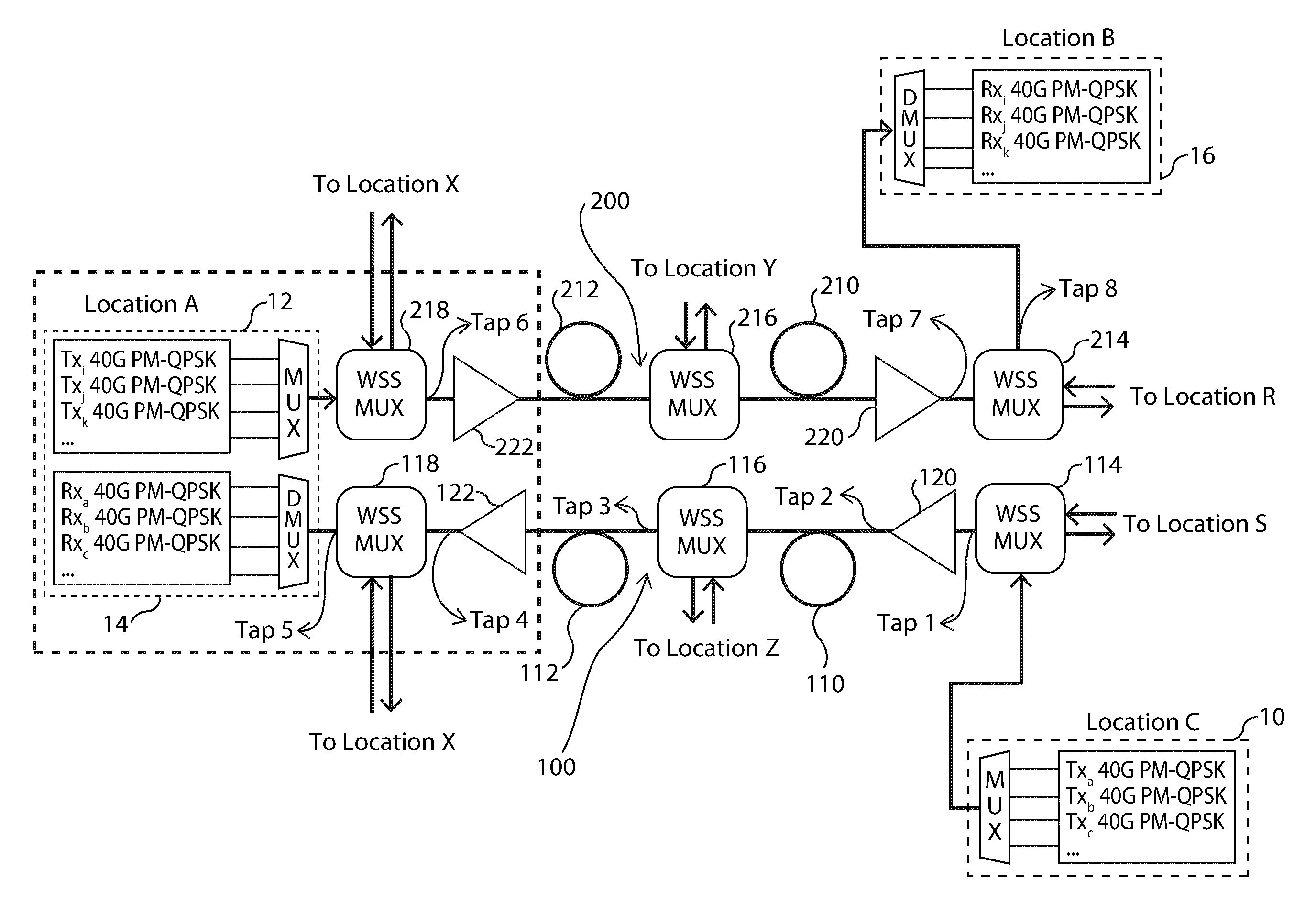
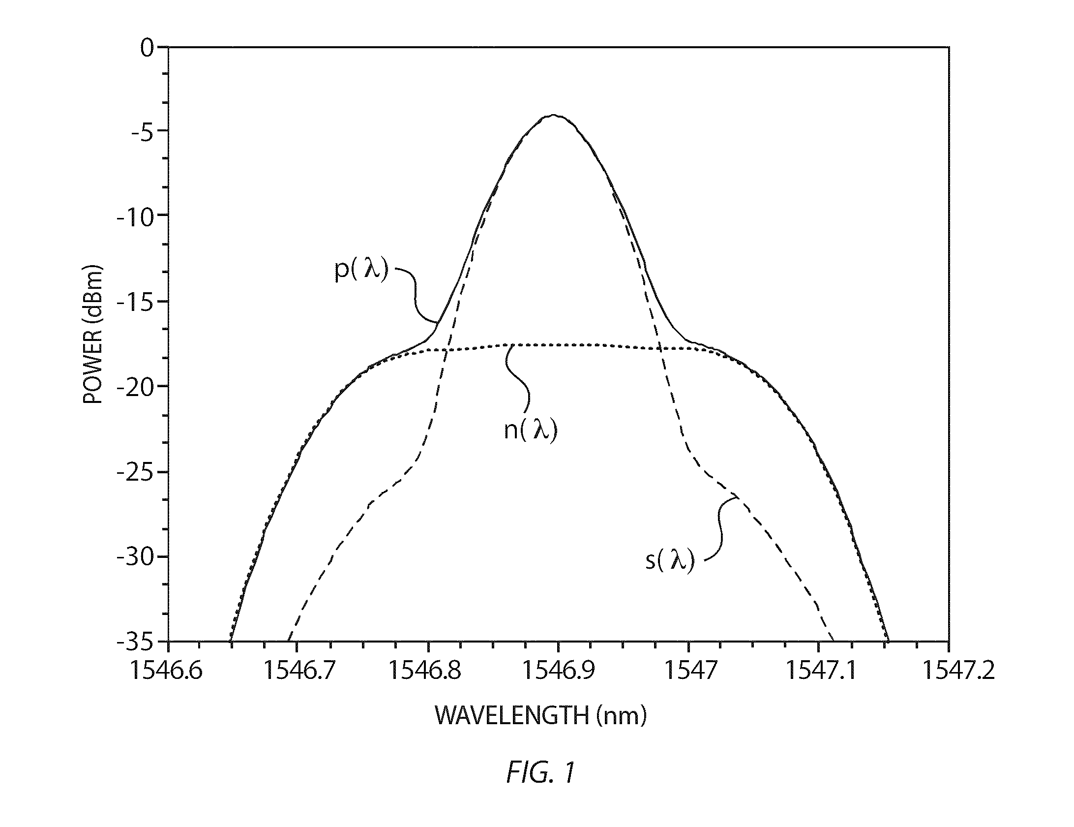
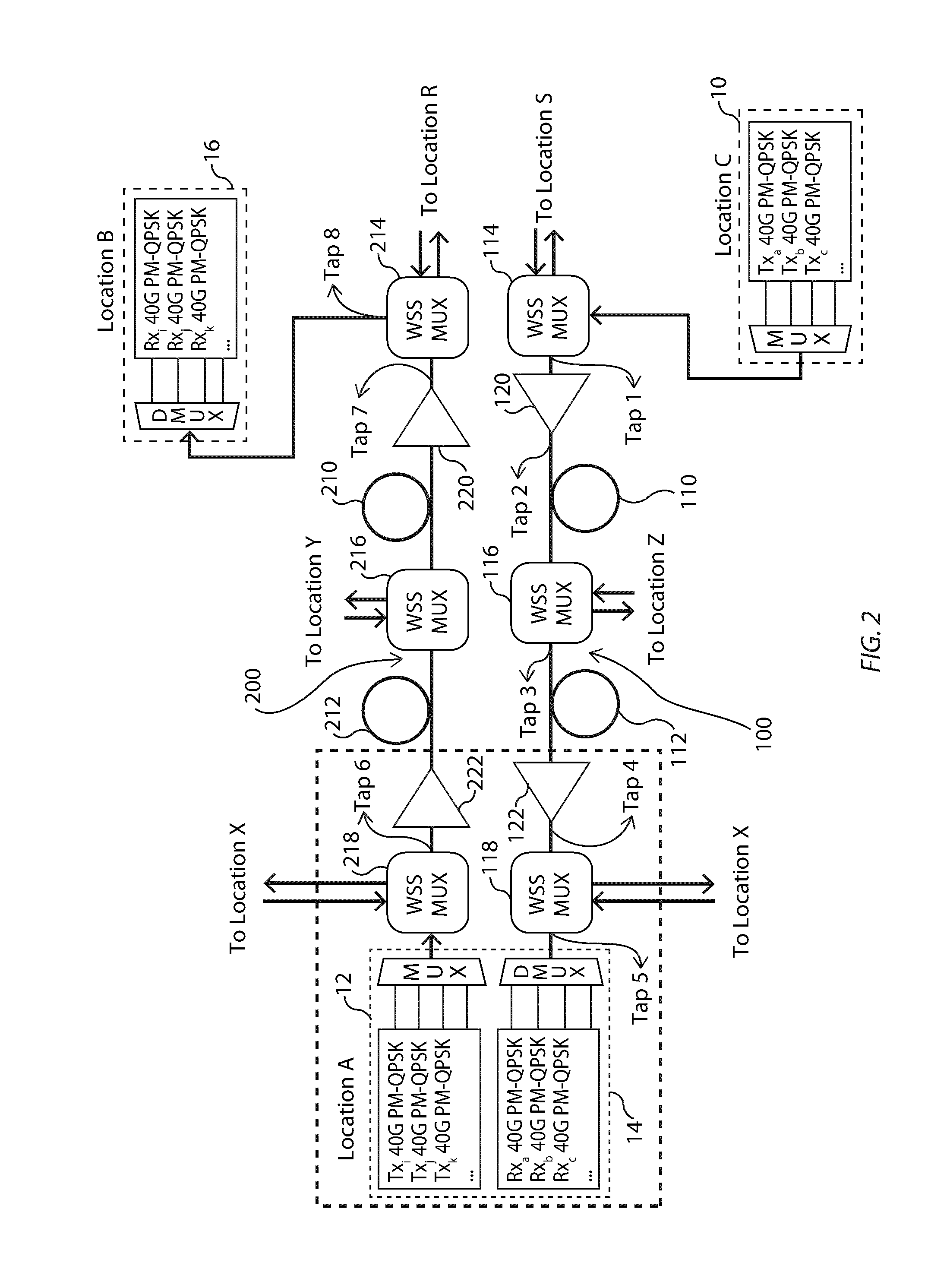
[0065]FIG. 5 illustrates an embodiment of a processing algorithm used to estimate the noise contribution on the trace P(λ) of the SUT obtained at Tap 3, using the reference trace R(λ) obtained at Tap 1. The processing algorithm is based on the method of FIG. 4. In this example case, the spectral shape Sh(λ) corresponds to the reference trace R(λ) (step 406). The ratio K is estimated by calculating the ratio between the maximum value of trace P(λ) and the maximum value of the reference trace R(λ) (step 408):
K=max(P(λ)) / max(R(λ))
[0066]In this case, K=4.426. The spectrally-resolved trace of the signal contribution and the noise contribution of the SUT are respectively the estimated as follows (step 410):
Se(λ)=K·R(λ)
Ne(λ)=P(λ)−K·R(λ)
[0067]In is noted that because this estimation of K assumes a negligible noise contribution on trace P(λ) of the SUT at the peak wavelength, the estimation of the noise contribution Ne(λ) cannot be valid at wavelengths in the vicinity of the peak wavelength....
example 2
[0069]It is noted that this processing algorithm does not necessarily require a spectral-resolved point-by-point analysis. In a second example embodiment, data is obtained at three different resolution bandwidths, for example the “physical resolution” of the OSA, a 0.1-nm resolution bandwidth and a 0.2-nm resolution bandwidth.
[0070]This example also assumes a negligible noise contribution on the reference signal such that Sh(λ)=R(λ) (step 406).
[0071]The process is then as follows:
[0072]The reference trace R(λ) is acquired (in this example, at Tap 1) and the peak power R(λpk) is determined.
[0073]A second R0.1(λ) and a third R0.2(λ) reference traces are obtained either by performing additional acquisitions of the reference signal using respectively a first and a second resolution bandwidth RBW1, RBW2, e.g. 0.1-nm and 0.2-nm resolution bandwidths in this case, or by integrating trace R(λ) in software. The peak powers of these traces R0.1(λpk), R0.2(λpk) are then determined.
[0074]The tr...
example 3
[0081]FIG. 6 illustrates another embodiment of a processing algorithm used to estimate the noise contribution on the trace P(λ) of the SUT obtained at Tap 3, using the reference trace R(λ) obtained at Tap 1. The processing algorithm is based on the method of example 1 but uses a different processing algorithm to estimate the ratio K.
[0082]This example also assumes a negligible noise contribution on the reference signal such that Sh(λ)=R(λ) (step 406).
[0083]This processing algorithm is made using measurements made at two distinct wavelengths λ1 and λ2 that are within the optical signal bandwidth of the SUT and generally positioned on the same side of the peak of the SUT. By assuming a uniform noise distribution within the optical signal bandwidth and therefore a substantially equal noise level at λ1 and λ2 on the trace P(λ) and trace R(λ), we find:
P(λ2)-P(λ1)=S(λ2)-S(λ1)=S(λ1)(S(λ2)S(λ1)-1)=S(λ1)(R(λ2)R(λ1)-1)=S(λ1)R(λ1)(R(λ2)-R(λ1))
and the ratio K is then estimated in the region aro...
PUM
 Abstract
Description
Claims
Application Information
 - R&D Engineer
- R&D Manager
- IP Professional
- Industry Leading Data Capabilities
- Powerful AI technology
- Patent DNA Extraction
Browse by: Latest US Patents, China's latest patents, Technical Efficacy Thesaurus, Application Domain, Technology Topic.
© 2024 PatSnap. All rights reserved.Legal|Privacy policy|Modern Slavery Act Transparency Statement|Sitemap