Maximum load supply capability evaluation method of medium-voltage power distribution network for loop power supply

[0076] The technical solutions in the embodiments of the present invention will be clearly and completely described below in conjunction with the drawings in the embodiments of the present invention.

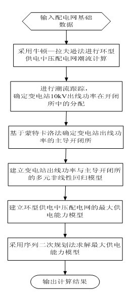
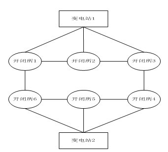
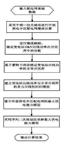
[0077] The present invention proposes a maximum power supply capacity model of a ring-type power supply medium voltage distribution network based on a multivariate nonlinear regression curve model. The flowchart of the embodiment is as follows figure 1 Shown, now figure 2 The illustrated example network is taken as an example for explanation:

[0078] Step 1. Enter the basic data of the ring-type power supply medium voltage distribution network:

[0079] Generally in a ring-type power supply medium-voltage distribution network, including substations, power plants, switching stations, etc., the basic data includes system lines and unit, switching station loads, transformers and other component parameter information. When dealing with the actual grid, in addition to the medium-voltage distribution network, the lines and units in the high-voltage distribution network should also be input in the model.

[0080] The research objects in the examples are figure 2 As shown, it is a ring-type power supply 10kV medium voltage distribution system including 2 110kV substations and 6 switching stations, which are respectively denoted as substation 1, substation 2, switching substation 1, switching substation 2, switching substation 3 , Opening and closing station 4, opening and closing station 5, opening and closing station 6. Opening and closing station 1, opening and closing station 2, opening and closing station 3, opening and closing station 4, opening and closing station 5, and opening and closing station 6 are connected in a loop, and substation 1 is connected to opening and closing station 1, opening and closing station 2, and opening and closing station 3. The substation 2 is connected to the opening and closing station 4, the opening and closing station 5, and the opening and closing station 6. Establish a basic database including line parameters, main transformer parameters of the substation, load of switching stations (system load parameters of the embodiment), and normal operation mode of the system. The normal operation mode of the system refers to the actual operation state of the system grid for which the maximum load capacity is to be sought. For example, a distribution network with a ring grid structure, the normal operation mode of the system is open loop operation or closed loop operation. The basic data involved in the embodiment is shown in Table 1-3:

[0081] Table 1 Line parameters

[0082]

[0083] Table 2 Load parameters of opening and closing

[0084]

[0085] Note: The reactive power is selected according to the power factor of 0.95

[0086] Table 3 Substation parameters

[0087]

[0088]

[0089] Step 2: According to the basic data described in Step 1, the power flow calculation of the ring-type power supply medium voltage distribution network is performed. The power flow calculation methods that can be used in the present invention include Newton-Raphson method, PQ decomposition method, etc. In the embodiment, Newton-Raphson method is used for ring-type power supply and medium-voltage distribution network for power flow calculation, Newton-Raphson method is an existing technology . The Newton-Raphson method is used to calculate the power flow equation of the example. The active power results of each branch are shown in Table 4.

[0090] Table 4 Branch circuit active power

[0091]

[0092] For the convenience of implementation and reference, the following is a detailed description of the use of Newton-Raphson method for power flow calculation of ring-type power supply and medium-voltage distribution network.

[0093] (1) Basic equation of tidal current

[0094] Equation (2.1) gives the mathematical equation of the tidal current equation,

[0095] P i - jQ i V ^ · = X i = 1 n Y ij V · j ( i , j = 1,2,3 , . . . , n ) - - - ( 2.1 )

[0096] V imin ≤V i ≤V imax (2.2)

[0097] P Gimin ≤P Gi ≤P Gimax (2.3)

[0098] Q Gimin ≤Q Gi ≤Q Gimax (2.4)

[0099] |δ i -δ j | i -δ j | max (2.5)

[0100] Among them, (2.1) is the basic equation for power flow calculation, and (2.2) is the node voltage constraint. Equations (2.3) and (2.4) are the constraints on the active power and reactive power of the power supply nodes in the network, and equation (2.5) is the power angle constraint between nodes; P i , Q i Refers to the active power and reactive power of the i-th node, Refers to the voltage vector of the jth node, Means Conjugate, Y ij Refers to the mutual admittance between the i-th node and the j-th node. V i , V imin And V imax Respectively are the i-th node voltage and its upper and lower limit vectors; P Gi , P Gimin And P Gimax Are the active power of the i-th node and its upper and lower limit vectors; Q Gi , Q Gimin And Q Gimax Are the reactive power of the i-th node and its upper and lower limit vectors; |δ i -δ j |and|δ i -δ j | max Is the power angle difference and the upper limit of the power angle difference between the i-th node and the j-th node. The node referred to in the present invention is a power node with a generator, and is also called a bus in the art.

[0101] (2) Basic principles of Newton Newton-Raphson method

[0102] Take solving the nonlinear equation f(x)=0 as an example to illustrate the basic principle of Newton's method. When solving this equation, first take the initial value x near the true value (0) , Let x = x (0) +Δx (0) , Δx (0) X (0) The correction amount. F(x (0) +Δx (0) )=0 at x (0) Near Tyler expands:

[0103] f ( x ( 0 ) + Δx ( 0 ) ) = f ( x ( 0 ) ) + f ′ ( x ( 0 ) ) * Δx ( 0 ) + f ′ ′ ( x ( 0 ) ) * ( Δx ( 0 ) ) 2 2 ! + . . . + f n ( x ( 0 ) ) * ( Δx ( 0 ) ) n n ! + . . . ( 2.6 )

[0104] When Δx (0) When the value is very small, the second-order derivative term and higher-order derivative term in equation (2.6) can be ignored, and equation (2.6) is transformed into:

[0105] f(x (0) +Δx (0) )=f(x (0) )+f′(x (0) )*Δx (0) = 0

[0106] which is:

[0107] f(x (0) )=-f′(x (0) )*Δx (0) (2.7)

[0108] Get about Δx (0) The modified equation of, solve this equation can get Δx (0). Use formula x = x (0) +Δx (0) Corrected initial value x (0) To get the new initial value x (1) , And then find the new correction Δx (1) , And so on repeatedly until the convergence criterion is met, that is, the numerical solution of the original equation is obtained.

[0109] (3) Calculation steps of Newton-Raphson method

[0110] When calculating power flow, first input the original data of the network and the given value of each node to form the node admittance matrix. Based on voltage vector During the iteration process, the real part of the k-th node voltage value is denoted as e (k) , The imaginary part of the kth node voltage value is denoted as f (k) , The initial value of the input node voltage value e (0) And f (0) (Without subscripts, it means the vector composed of the voltage values ​​of all nodes), and set the iteration count k=0. Then start the iteration, the iteration process is as follows:

[0111] 1) The node voltage value e calculated from the previous iteration (k-1th) (k) And f (k) (When k=0, it is the given initial value e (0) And f (0) ), calculate the current (kth) imbalance of each node (including substation bus and switching station bus) with among them Is the unbalanced amount of active power of the i-th node, Is the unbalanced amount of reactive power of the i-th node, Is the unbalanced amount of the square of the voltage of the i-th node.

[0112] 2) Check the convergence according to the following conditions,

[0113] max { | ΔP i ( k ) , ΔQ i ( k ) , ΔV i 2 ( k ) | } ϵ - - - ( 2.8 )

[0114] If it converges, the iteration ends here, transfer to the calculation of the power flow of each line and the power of the balance node, and print out the calculation results. If it does not converge, continue to calculate. ε is the preset threshold, and it is sufficient to set a sufficiently small amount in specific implementation.

[0115] 3) Calculate each element of the Jacobian matrix for writing the correction equation, and the specific calculation belongs to the prior art.

[0116] 4) Write the correction equation according to the Jacobian matrix to find the correction value of the node voltage value with The specific implementation method belongs to the prior art.

[0117] 5) Correct the voltage of each node, the voltage correction formula of the i-th node is as follows

[0118] e i ( k + 1 ) = e i ( k ) + Δe i ( k ) , f i ( k + 1 ) = f i ( k ) + Δf i ( k ) - - - ( 2.9 )

[0119] 6) Iterative calculation adds 1 and returns 1) Continue the iterative process.

[0120] After the iteration, the power of the balance node and the power distribution in the network must be calculated (see Table 4). The voltage of the balance node remains the same during the iteration process, and is a node where the voltage remains the same.

[0121] If used Represents the line current I from the i-th node to the j-th node ij The formula for calculating the power of the transmission line is as follows:

[0122] S ij = P ij + j Q ij = V · i I ^ ij = V i 2 y ^ i 0 + V · i ( V · i - V · j ) y ^ ij - - - ( 2.10 )

[0123] S ij : Apparent power of the line from the i-th node to the j-th node

[0124] P ij : Active power of the line between the i-th node and the j-th node

[0125] Q ij : Reactive power of the line from the i-th node to the j-th node

[0126] Voltage phasor of the i-th node

[0127] Ground admittance of the i-th node

[0128] Voltage phasor of the jth node

[0129] Admittance of the line from the i-th node to the j-th node

[0130] The value of i is 1, 2, ..., n, the value of j is 1, 2, ..., n, i≠j, and n is the total number of nodes.

[0131] Step 3. On the basis of the results of the power flow calculation in step 2, perform power flow tracking to determine the distribution of the 10kV outgoing line power of each substation in the ring-type power supply medium voltage distribution network in the switching station and the switching station to the 10kV outgoing line of the substation Power draw situation.

[0132] In the embodiment, based on the power flow calculation result in step 2, the power loss of the line is equivalent to the load at both ends of the line, the ring network is treated as a lossless network, and the power flow tracking results are shown in Table 5.

[0133] Table 5 Power distribution of 10kV outgoing line to load in substation (MW)

[0134]

[0135]

[0136] From Table 5, we can see the power draw of the switching station and the power distribution of the substation. For example, switching station 2 draws 5.4747MW active power and 2.1253MW active power from line 2 and substation 2 respectively, and the total active power drawn is 7.6MW, which is equal to the total active power brought by the switching; the power distribution of line e The active power of switching station 1 is 0.0362MW, the active power of switching station 5 is 7.0648MW, the active power of switching station 6 is 0.8979MW, and all the power of the substation is allocated to the switching station load; other switching stations The power drawn and the power allocated by the substation are shown in Table 5.

[0137] The present invention further provides a method for realizing power flow tracking, including the following sub-steps:

[0138] 1) According to the power flow results of the normal state system calculated in step 2, a lossless network is formed;

[0139] 2) Form the downstream distribution matrix A and node active power matrix P based on the lossless network LL And node total injected active power matrix P TT;

[0140] 3) Calculate the inverse matrix of the downstream distribution matrix A, and calculate the load of the switching station to the branch power draw coefficient matrix K L =P LL (P TT A T ) -1;

[0141] 4) Assuming that a certain switching station is the i-th node, the connection between the s-th node and the t-th node constitutes a branch s-t, and calculate the load P of the i-th node to the line power Li-st =k Li tP st;

[0142] Where P Li-st Refers to the active power draw of the branch s-t by the load of the i-th node, K L =(k Lit ) n×n Element k Lit Refers to the distribution coefficient matrix of the load of the i-th node to the branch s-t, P st Refers to the active power of the branch s-t.

[0143] For ease of implementation and reference, specific instructions for power flow tracking are provided as follows:

[0144] (3.1) The specific method of establishing the downstream distribution matrix is:

[0145] The equivalent value of the research object is the lossless network, and the downstream distribution matrix between nodes is established based on the results of the power flow calculation A=(a ij ) n×n

[0146]

[0147] The line from the i-th node to the j-th node can be denoted as line i-j.

[0148] In the formula P ij (≥0) is the active power transmitted from the i-th node to the j-th node, P Tj Inject the total active power for the jth node.

[0149] The downstream distribution matrix between nodes contains information such as the connection relationship between nodes, the direction of branch active power flow, and the size of node injection power.

[0150] (3.2) The specific method of establishing the load and line power flow tracking analytical model of the switching station is:

[0151] The relationship between the switching load and the 10kV outlet power of the substation is

[0152] P Li-st =K L P st (3.2)

[0153] Suppose the i-th node is a load node, and the s-th node and the t-th node in the network are connected to form a branch s-t.

[0154] Where P Li-st Refers to the active power draw of the branch s-t by the load of the i-th node, K L =(k Lit ) n×n Element k Lit Refers to the distribution coefficient of the load of the i-th node to the branch s-t, P st Refers to the active power of the branch s-t. In the embodiment, the node where the load exists is the switching station.

[0155] Switching station load to line power draw coefficient matrix K L =(k Lit ) n×n for

[0156] K L =P LL (P TT A T ) -1 (3.3)

[0157] P LL =diag(P L1 , P L2 ,...P Ln ) (3.4)

[0158] P TT =diag(P T1 , P T2 ,...P Tn ) (3.5)

[0159] Where P Li Is the active power of the i-th node, P LL Is an n×n-dimensional node active power matrix, where P L1 , P L2 ,...P Ln Are the active power of nodes 1, 2, ..., n; P Ti Is the total injected active power of the i-th node, P TT Is an n×n-dimensional node total injected active power matrix, where P T1 , P T2 ,...P Tn They are the total injected active power of the first, second, ..., n nodes, where n is the total number of nodes; formula (3.2) reflects the qualitative relationship between the switching load and the line power, that is, the switching load The drawing of the required power to the power of each line and the distribution of the power of each line in each switching station. The active power drawn by the switching station i to the branch s-t is

[0160] P Li-st =k Lit P st (3.6)

[0161] Step 4, using the results of the power flow calculation in step 2 and the power flow tracking results obtained in step 3 as the initial point, within the load capacity range of the switching station, the Monte Carlo method is used to determine the multi-group load distribution of the switching station in the ring network. The load distribution of each group of switching stations is calculated and tracked separately to obtain multiple sets of power flow tracking results, and the dominant switching station for the 10kV outlet power of the substation is determined.

[0162] The dominant switching stations are those that have a greater impact on the active power of a certain line. Based on the results of the power flow analysis, the power flow tracking theory can be used to determine the distribution of the 10kV outgoing line power of the ring-shaped substations in the switching load and the drawing of the switching load to the 10kV outgoing line of the substation. Taking this as the initial point, the Monte Carlo method of switching load parameter perturbation is used to determine the dominant switching station for the 10kV outlet power of the substation. The Monte Carlo method is the prior art, and the present invention will not repeat it.

[0163] Table 6 shows the main opening and closing positions of the 10kV outlet power of the substation obtained in the embodiment.

[0164] Table 6 Leading opening and closing stations of substation outlets

[0165] Busbar

[0166] Step 5: Based on the multiple sets of power flow tracking results obtained in Step 4, establish a multiple nonlinear regression model between the 10kV outgoing power of the substation and the main switching station. Based on the results of power flow tracking, the embodiment obtains a multivariate nonlinear regression model between the 10kV outlet of each substation and the main switching station through least squares estimation and fitting. Since the accuracy of the quadratic polynomial is sufficiently high, the quadratic polynomial is adopted.

[0167] (5.1) Suppose a certain switching station is the i-th node, denoted as switching station i, and the power flow tracking nonlinear curve model of the power drawn by the switching station i to line l is

[0168] P l - Li = a 0 + a 1 P Li + a 2 P Li 2 + . . . + a t P Li t - - - ( 5.1 )

[0169] Where P l-Li Is the power drawn from line l for switching; P Li Is the load of opening and closing position i; a 0 , A 1 ,...A t Is the regression coefficient; t is the number of tidal current tracking curves. The value of L can be 1, 2,...L, where L is the total number of lines. In this embodiment, in order to facilitate the identification of nodes, the value of the line label l is a, b, c, d, e, f.

[0170] (5.2) Multivariate power flow tracking nonlinear curve model of the load of switching station i to the power drawn by line l

[0171] The power draw of the load of the switching station i to the line l is not only related to the load it is in, but also related to the loads carried by other switching, that is, the power draw of the load of the switching station i to the line l is related to all switching and There is a non-linear relationship:

[0172] P l - Li = X k = 1 m ( a ik 1 P Lk 1 + a ik 2 P Li 2 + . . . + a ikt P Lit ) + a 0 - - - ( 5.2 )

[0173] Where m is the number of opening and closing positions, K is the power of t with load, a ikj , J = {1, 2,..., t} represents P in the multivariate power flow tracking nonlinear curve model of the power drawn by the switch i load to line l Lit The coefficient of the term, a 0 It is a constant term coefficient, and k represents the kth load of the loop-type power grid. In the embodiment, the loads are provided by switching, so the value of k is 1, 2, ... m.

[0174] (5.3) Multivariate nonlinear regression model of line power and dominant switching station

[0175] At the same time, it can be known from the power flow tracking theory that the power of line 1 is all allocated to the leading switching station, and the power of line 1 is

[0176] P Pl = X f = 1 n z P l - Lf = X f = 1 n z ( X k = 1 m ( a fk 1 P Lk 1 + a fk 2 P Lf 2 + . . . + a fkt P Lft ) + a 0 )

[0177] = X k = 1 m ( P Lk 1 X f = 1 n z a fk 1 + P Lf 2 X f = 1 n z a fk 2 + . . . + . . . P Lft X f = 1 n z a fkt ) + a ^ 0 - - - ( 5.3 )

[0178] = X k = 1 m a ^ k 1 P Lk 1 + a ^ k 2 P Lk 2 + . . . + a ^ kt P Lkt + a ^ 0

[0179] Where P l-Lf Is the power drawn from line l for the f-th dominant switch, n z Is the number of leading openings, Is the estimator of the coefficient of the constant term, j={1, 2,..., t} is the estimator of the regression coefficient. a ikj , J = {1, 2,..., t}, P Lkt The meaning is the same as the 5.2 formula.

[0180] The specific implementation of the embodiment is as follows:

[0181] The objective function of the traditional maximum power supply capacity is the maximum sum of the switching loads in the network, as shown in the following formula,

[0182] MLSC = X i P Li

[0183] For the ring-shaped power supply and distribution network shown in the calculation example, there is no power supply in the system, (if it contains power, the node is processed as a load that emits power), then the sum of the power of the substation off the grid and the power of the 10kV outgoing line of the substation is equal to the switching station The sum of loads is shown in the following formula.

[0184] P a +P b +P c +P d +P e +P f =P L2 +P L3 +P L4 +P L5 +P L6 +P L7

[0185] The maximum power supply capacity of the ring system shown in the calculation example can be equivalent to the maximum power supply capacity of the 10kV substation outgoing line without considering the network loss, that is, the maximum power supply capacity of the ring-shaped distribution network is transformed into the 10kV outgoing line of the substation Is the objective function of the variable, as shown in the following formula.

[0186] MLSC = X i P Li = X l P Pl ( l = a , b , c , d , e , f )

[0187] In step 5, the multiple regression models of the 10kV outgoing line of each substation and the main switching station are obtained:

[0188] P Pl = X k = 1 m a ^ k 1 P Lk 1 + a ^ k 2 P Lk 2 + . . . + a ^ kt P Lkt + a ^ 0 ( l = a , b , c , d , e , f )

[0189] The coefficients of the multiple regression model of the 10kV substation and the main switching station are shown in Table 7:

[0190] Table 7 Multiple regression model parameters of line a and leading opening and closing station

[0191]

[0192]

[0193] That is, the multiple regression model of line a and the main opening and closing station is shown in the following formula

[0194] P Pa = 0.4227 P L 1 + 0.0044 P L 1 2 + 0.2164 P L 2 - 0.0112 P L 2 2 + 0.0847 P L 3 +

[0195] 0.0186 P L 3 2 + 0.1656 P L 6 + 0.0082 P L 6 2

[0196] In the same way, the multiple regression models of the other 5 10kV substation outlets and the corresponding leading opening and closing stations can be obtained

[0197] Table 8 Multiple regression model parameters of line b and leading opening and closing station

[0198]

[0199] That is, the multiple regression model of line b and the main opening and closing station is shown in the following formula

[0200] P Pb = 0.1609 P L 1 - 0.0051 P L 1 2 + 0.3270 P L 2 + 0.0060 P L 2 2 + 0.1252 P L 3 -

[0201] 0.0106 P L 3 2

[0202] Table 9 Multiple regression model parameters of line c and leading opening and closing station

[0203]

[0204] That is, the multiple regression model of line c and the main opening and closing station is shown in the following formula

[0205] P Pc = 0.1170 P L 1 + 0.0040 P L 1 2 + 0.2286 P L 2 - 0.0123 P L 2 2 + 0.5034 P L 3 +

[0206] 0.0064 P L 3 2 + 0.1734 P L 3 - 0.0072 P L 4 2

[0207] Table 10 Multiple regression model parameters of line d and leading opening and closing station

[0208]

[0209] That is, the multiple regression model of line d and the main opening and closing station is shown in the following formula

[0210] P Pd = 0 . 0809 P L 2 - 0.0080 P L 2 2 + 0 . 1545 P L 3 + 0.0068 P L 3 2 + 0 . 4517 P L 4 +

[0211] 0.0025 P L 4 2 + 0.2107 P L 5 + 0.0021 P L 5 2 + 0.0844 P L 6 - 0.0844 L 6 2

[0212] Table 11 Multiple regression model parameters of line e and leading opening and closing station

[0213]

[0214] That is, the multiple regression model of line e and the main opening and closing station is shown in the following formula

[0215] P Pe = 0.2134 P L 4 - 0.2145 P L 4 2 + 0.4662 P L 5 - 0.0023 P L 5 2 + 0.1651 P L 6 +

[0216] 0.0074 P L 6 2

[0217] Table 12 Multiple regression model parameters of line f and leading opening and closing station

[0218]

[0219] That is, the multiple regression model of line f and the main opening and closing station is shown in the following formula

[0220] P Pf = 0.1721 P L 1 - 0.0316 P L 1 2 + 0.0915 P L 2 + 0.0052 P L 2 2 + 0.0701 P L 4 -

[0221] 0.0066 P L 4 2 + 0.1384 P L 5 - 0.0025 P L 5 2 + 0.4515 P L 6 - 0.0065 P L 6 2

[0222] Step 6. Based on the multiple nonlinear regression model obtained in Step 5, establish the maximum power supply capacity model of the ring-type power supply medium voltage distribution network:

[0223] The ring-type distribution network also needs to meet the power flow balance, which is described by the relationship between the node current I and the node voltage V, namely:

[0224] I=YV

[0225] Among them, Y is the nodal admittance matrix. Here, the node current I and the node voltage V are the current matrix and the voltage matrix of all n nodes.

[0226] At the same time, considering the "N-1" power supply requirements of the power grid and the thermal stability requirements of the line, the power upper limit of the branch is considered to be half of the thermal stability limit capacity of the line and multiplied by a correction coefficient re; the lower limit considers the economic load rate of the line. As shown in the following formula

[0227] P i min ≤ P i ≤ P i max P i min = P E P i max = re 1 2 P H

[0228] Where P E Is the power corresponding to the economic load rate of the line, P H It is the thermal stability limit of the circuit.

[0229] For the switching stations in the actual distribution network, due to the different specifications and capacities and the regional loads provided by each switching station, the load carried by the switching stations meets the conditions as shown in the following formula:

[0230] P Limin ≤P Li ≤P Limax

[0231] Where P Li Refers to the active load of the i-th node, P Limin And P Limax Refers to the upper and lower limits of the active load of the i-th node. The voltage of the i-th node meets the upper and lower limits of the node voltage, that is

[0232] U imin ≤U i ≤U imax

[0233] Therefore, the model of the maximum power supply capacity of the ring distribution network formed by the above formulas is shown in formula (6.1):

[0234] max MLSC = X i P Li = X l P Pl

[0235] s . t . P i = X k = 1 m a k 1 P Lk 1 + a k 2 P Lk 2 + . . . + a kt P Lkt I = YV P Li min ≤ P Li ≤ P Li max P i min ≤ P i ≤ P i max U i min ≤ U i ≤ U i max - - - ( 6.1 )

[0236] In the formula: when the i-th node is a substation, satisfy P imin ≤P i ≤P imax , P imin , P imax For the actual active power of the 10kV outgoing line of the i-th node (substation) and its upper and lower limits, there are A total of outgoing lines in the relevant substation;

[0237] U i , U imin , U imax Is the bus voltage of the i-th node and its upper and lower limits, set a total of B bus voltages to be investigated;

[0238] When the i-th node is the opening and closing position, satisfy P Liminn ≤P Li ≤P Limax , P Li , P Limin , P Limax For the actual load of the i-th node (switching station) and its upper and lower limits, there are a total of C switches on the ring.

[0239] Step 7: Solve the global optimal solution of the maximum power supply capacity model, obtain the maximum power supply capacity model of the ring power supply medium voltage distribution network, and obtain the maximum power supply capacity of the ring power supply medium voltage distribution network according to the maximum power supply capacity model.

[0240] The nonlinear constrained optimization problem shown in equation (6.1) can be simplified as follows. The equality constraint has been embodied in the multivariate nonlinear regression model. The inequality constraint in equation (6.1) is transformed into a simple inequality g i (P L )≥0, i∈I={1,2,...,A+B+C}, where P L For the node load vector, the maximum common possibility can be expressed as follows:

[0241] min f ( P L ) = - 1 * f MLSC ( P L ) = - 1 * X i = 1 C P L , s . t . g i ( P L ) ≥ 0 , i A I = { 1,2 , . . . , A + B + C } ,

[0242] Newton-Lagrangian, SQP, trust region, intelligent algorithm and other methods can be used to solve the global optimal solution of the maximum power supply capacity model. The embodiment adopts a sequential quadratic programming method to obtain the optimal solution of the maximum power supply model of the ring-type power supply medium-voltage distribution network corresponding to formula (6.1), which can quickly converge. The model is solved below based on the sequential quadratic programming method.

[0243] At a given point (P L(k) , Μ k )(μ represents the Lagrangian multiplier, k represents the kth iteration, P L(k) Represents P of the kth iteration L , Μ k After representing the Lagrangian multiplier of the k-th iteration, the constraint function is linearized, and the Lagrangian function is approximated by a quadratic polynomial, and the following form of the quadratic programming sub-problem is obtained:

[0244] min 1 2 d T B k d + ▿ f ( P L ( k ) ) T d = 1 2 d T B k d + I T * d

[0245] s.t.g(P L(k) )+A k d≥0

[0246] Among them, I=-1*[1,1,...,1] T , B k Is the Lagrangian function L(P L(k) , Μ k ) Approximation of Hessian matrix, d is the value function φ(P L ,Μ,σ), and σ is the penalty factor.

[0247] The augmented Lagrangian value function φ(x, v, r) is used to improve the acceptance of the super-linear convergence step and overcome the Maratos effect. The expression is as follows:

[0248] φ ( P L , v , r ) = f ( P L ) - X j A J ( P L , μ ) ( μ j g j ( P L ) - 1 2 σ j g j 2 ( P L ) )

[0249] among them:

[0250] J(P L ,Μ)={j∈I|g j (P L )≤μ j /σ j }.

[0251] Just guarantee σ ≥ [ - ( d k y ) T A k W k Z k d k z - h ( P L ( k ) ) T ▿ μ ( P L ( k ) ) T d k | | g ( P L ( k ) ) | | 2 ] + δ ‾ , d k Is the value function φ(P Li , Μ, σ) of the falling direction.

[0252] Where Z k The column vector is the zero space N(A k ), G(P L(k) ) To P L(k) Jacobian matrix, d k Y component W k Is the Lagrangian function L(P L(k) , Μ k ) Hessian matrix.

[0253] In summary, the summary algorithm steps are as follows:

[0254] Step 0: Given the initial point (x 0 , Μ 0 )∈R n ×R n+m+l , Symmetric positive definite matrix B 0 ∈R n×n. Calculation

[0255] A 0 = ▿ g ( P L ( 0 ) ) T

[0256] Select parameter η∈(0,0.5), ρ∈(0,1), allowable error 0≤ε 1 , Ε 2 ≤1, let k:=0.

[0257] Step 1: Solve the sub-problems

[0258] min 1 2 d T B k d + ▿ f ( P L ( k ) ) T d

[0259] s.t.g(P L(k) )+A k d≥0

[0260] Get the optimal solution d k.

[0261] Step 2: If||d k || 1 ≤ε 1 , And ||(g k )-|| 1 ≤ε 2 , Stop the calculation, and get an approximate KT point (P Lk , Μ k ).

[0262] Step 3: For the value function φ(P L(k) ,Σ), select the penalty function σ k , Making d k Is the function in x k The direction of descent.

[0263] Step 4: Use the existing Armijio search method, the search method is, let m k Is the smallest non-negative integer m that makes the following inequality true:

[0264] φ(P L(k) +ρ m d k , Σ k )-φ(P L(k) , Σ k )≤ηρ m φ′(x k ,Σ;d k )

[0265] Let step factor Then P L(k+1) :=P L(k) +α k d k.

[0266] Step 5: Calculate the Jacobian matrix after the k+1 iteration:

[0267] A k + 1 = ▿ f ( x k + 1 ) T

[0268] And least squares multiplier μ k + 1 = [ A k + 1 A k + 1 T ] - 1 A k + 1 ▿ f k + 1

[0269] Step 6: Correction matrix B k For B k+1 ,make

[0270] s k =P L(k+1) -P L(k) =α k d k , y k = ▿ x L ( P L ( k + 1 ) , μ k + 1 , λ k + 1 ) - ▿ x L ( P L ( k ) , μ k + 1 , λ k + 1 ) ,

[0271] B k + 1 = B k - B k s k s k T B k s k T B k s k + z k z k T s k T z k

[0272] Where s k Is the search step length of step k, y k Is the increment of the Jacobian matrix, z k =θ k y k +(1-θ k )B k s k For B k The correction factor of the matrix.

[0273] Parameter θ k defined as

[0274]

[0275] Step 7: Let k:=k+1, go to step 1.

[0276] The embodiment compiles the SQP method calculation program according to the above steps, and the result is shown in (7.1):

[0277] MLSC=44.37MW (7.1)

[0278] At this time, the load carried by each switch and the power of the 10kV substation outgoing line are shown in Table (13) and Table (14) respectively.

[0279] Table 13 Loads of opening and closing at maximum power supply

[0280] Opening and closing

[0281] Opening and closing station 2

[0282] Table 14 Outgoing power of the substation at maximum power supply

[0283] Line

[0284] In summary, to figure 2 The calculation example system is given as an example to illustrate the calculation process of the maximum power supply capacity of the ring-type power supply medium-voltage distribution network based on the multiple nonlinear regression model in detail. It can be known from the results of the calculation examples that the present invention can solve the maximum power supply capacity model of the ring-type power supply and distribution network, the algorithm theory is solid, and the global optimal solution of the objective function can be obtained. At the same time, it can be concluded that when the network is at the maximum power supply capacity, the corresponding switching load and the power of the 10kV substation outgoing line can provide effective suggestions for the optimization and planning of the urban power grid.

[0285] Specific examples are used in this article to describe the principles and embodiments of the present invention. The description of the above embodiments is only used to help understand the method and core ideas of the present invention; at the same time, for those of ordinary skill in the art, according to this The idea of ​​the invention will change in the specific implementation and the scope of application. In summary, the content of this specification should not be construed as limiting the invention.