

Server performance prediction method based on particle swarm optimization nerve network
A particle swarm optimization and neural network technology, applied in the field of computer performance management, can solve problems such as loss of speed, inactivity, and difficulty in finding a global optimal solution, and achieve the effect of improving convergence and accuracy.
- Summary
- Abstract
- Description
- Claims
- Application Information
AI Technical Summary
Problems solved by technology
Method used
Image

Examples
Embodiment Construction
[0042] The technical scheme of the present invention is described in detail below in conjunction with accompanying drawing:
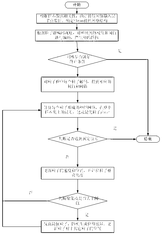
[0043] The present invention aims at the defect that in the existing particle swarm optimization neural network, the iterative update process of particle swarm is easy to fall into local optimum, improves the particle swarm optimization algorithm, and proposes a particle adjustment method based on particle swarm distribution. The main idea is that in each iteration In the process, when the distribution of the particle swarm is relatively dense, a random position increment is added to disperse the particles, thereby jumping out of the local optimal solution.
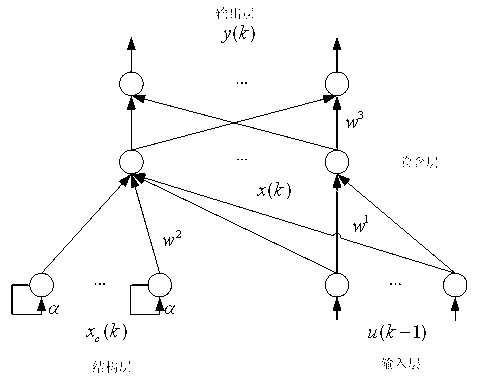
[0044] In order to facilitate the public to understand the technical solution of the present invention, the PSO-Elman neural network prediction model is taken as an example to describe in detail below.
[0045] Such as figure 1 As shown, the Elman neural network structure includes four layers: inp...
PUM
 Abstract
Description
Claims
Application Information