

A Computer Aided Design Method for Oval Curve in Road Route Design
A computer-aided, route design technology, applied in computing, special data processing applications, instruments, etc., can solve problems such as difficult to cut baselines, no application, difficult to establish equations that meet actual needs, etc.
- Summary
- Abstract
- Description
- Claims
- Application Information
AI Technical Summary
Problems solved by technology
Method used
Image

Examples
Embodiment 1
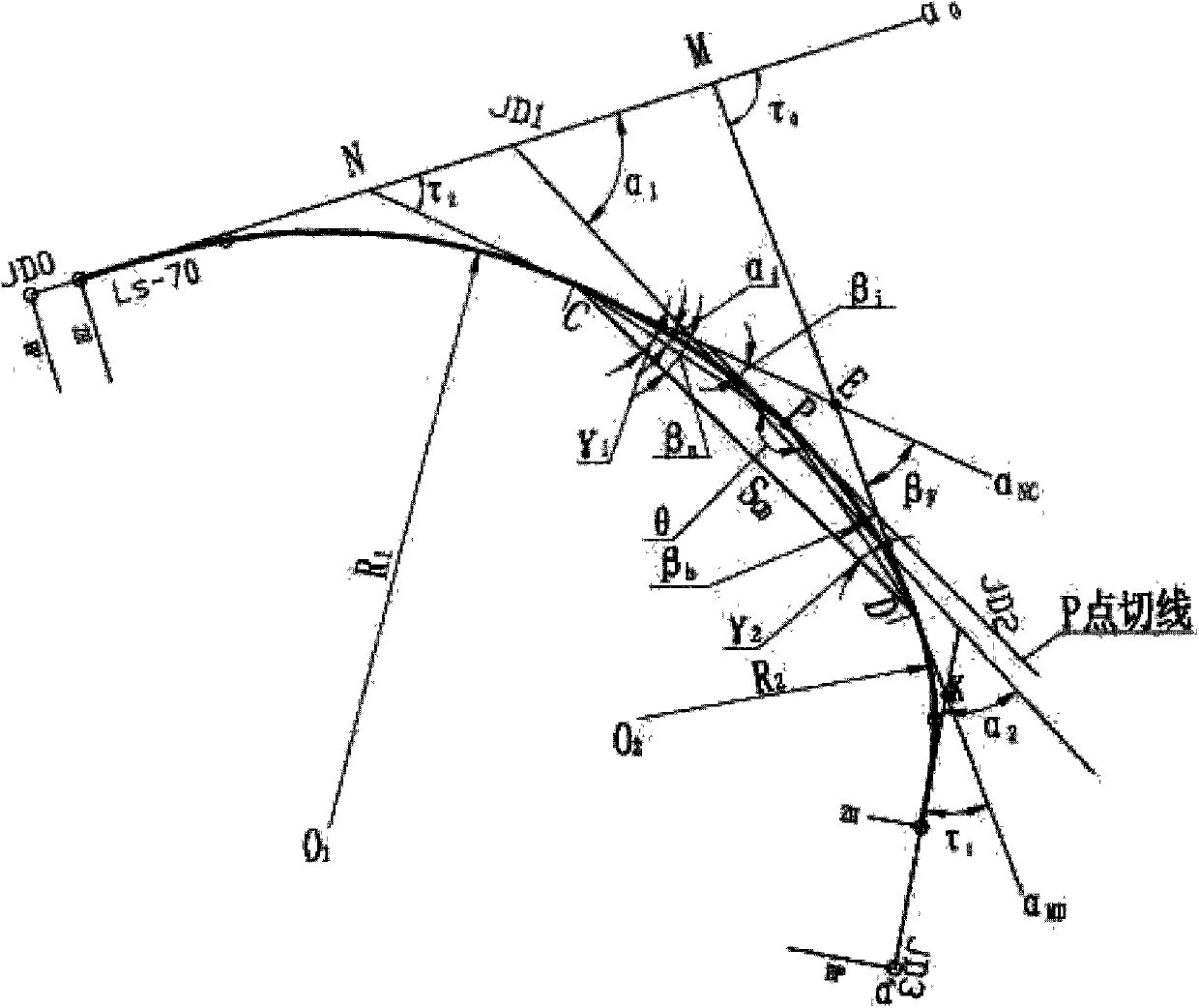
[0193] refer to figure 2 And Figure 5, the auxiliary design of modifying the C-shaped curve to an oval curve is as follows
[0194] JD 0 -JD 1 Azimuth α 0 =72°42′15"
[0195] JD 1 alpha 1 (Right)=64°40′36.4" R=275 LS1 =70
[0196] JD 2 alpha 2 (Right)=53°25′12.1" R=136.13687 L S2 =50
[0197] α'=α 0 +(α 1 +α 2 )=190°48′3.5"
[0198] It is currently a C-shaped curve.
[0199] JD 1 x 1 =600Y 1 =500;
[0200] JD 2 x 2 =376.7271616Y 2 =705.44701255.
[0201] Basic calculation:
[0202] P 1 =0.74242424 (R 1 +E 1 )=(R 1 +P 1 ) / cos(α 1 / 2)=326.3596195
[0203] P 2 =0.765161316 (R 2 +E 2 )=(R 2 +P 2 ) / cos(α 2 / 2)=153.2554885
[0204] Center coordinates: R 1 x 01 =284.8236392Y 01 =415.2977992
[0205] R 2 x 02 =334.7181487Y 02 =558.0615058
[0206] beta 01 =7°17′31.88" 3β 01 =21°52′35.65"
[0207] beta 02 =10°31′18.2" 3β 02 =31°33′54.61"
[0208] Design calculation process steps:
[0209] ①. Select point D on the small circle a...
Embodiment 2
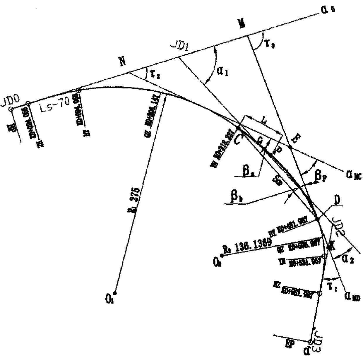
[0266] refer to image 3 and Figure 6 , the oval curve design of the latitude and longitude route design software is as follows
[0267] JD 0 -JD 1 Azimuth α 0 =39°09′16.4″
[0268] JD 1 alpha 1 (Right)=45°01′59.3″ R=330 L S1 =80
[0269] JD 2 alpha 2 (Right)=66°49′7.3" R=180.8389 L S2 =80
[0270] α'=α 0 +(α 1 +α 2 )=151°0′23″
[0271] JD 1 x 1 =394.6295Y 1 = 327.3237;
[0272] JD 2 x 2 =422.5821Y 2 = 601.9248.
[0273] Basic calculation:
[0274] P 1 =0.80808081 (R 1 +E 1 )=(R 1 +P 1 ) / cos(α 1 / 2)=358.106998
[0275] P 2 =1.474608984 (R 2 +E 2 )=(R 2 +P 2 ) / cos(α 2 / 2)=218.4028171
[0276] Center coordinates: R 1 x 01 =79.41003947Y 01 =497.2569625
[0277] R 2 x 02 =229.027493Y 02 =500.7496813
[0278] beta 01 =6°56′41.79" 3β 01 =20°50′5.37″
[0279] beta 02 =12°40′23.99" 3β 02 =38°01′11.97″
[0280] Design calculation process steps:
[0281] ①. Select point D on the small circle, in order to make R C with R 1 Clo...
Embodiment 3
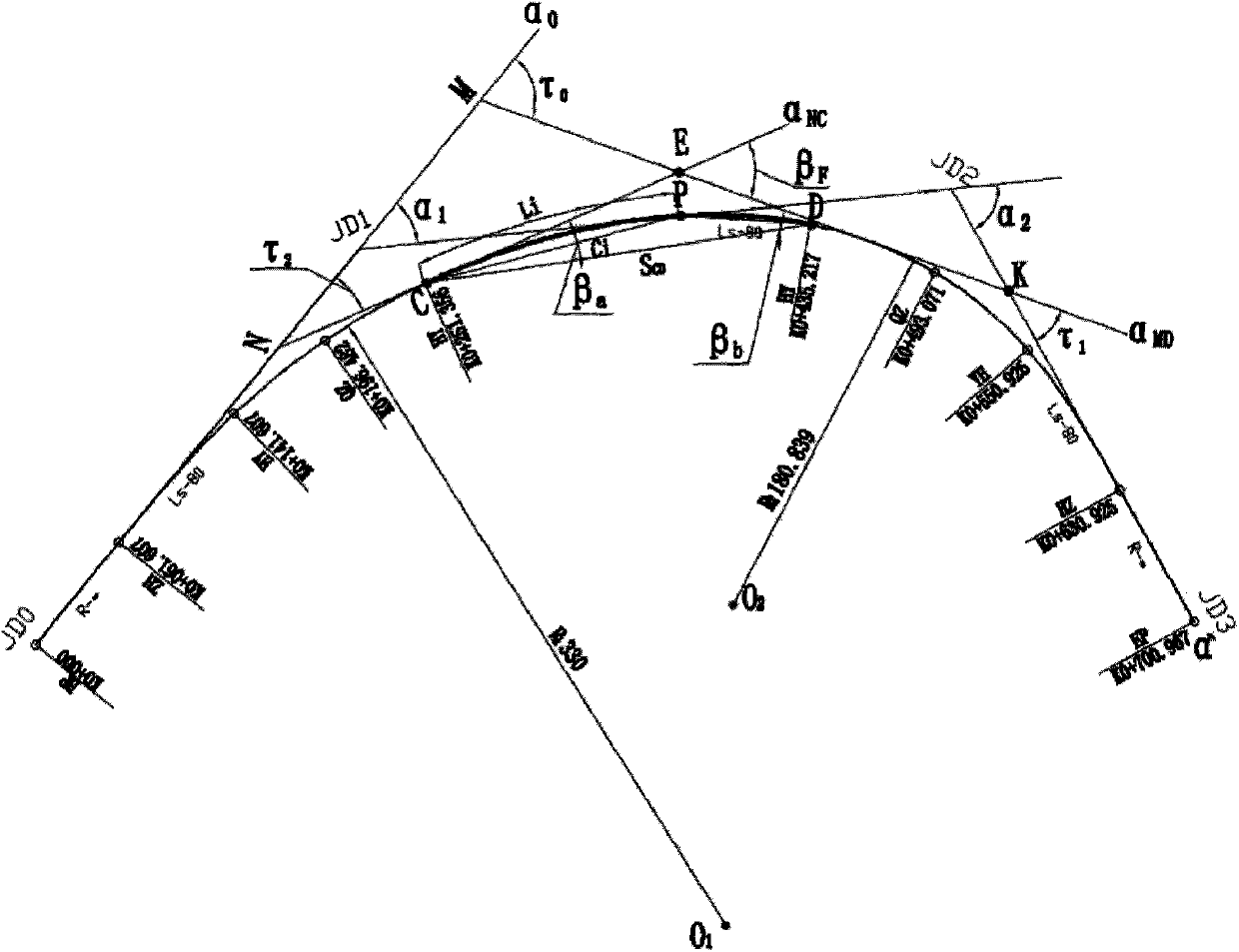
[0337] refer to Figure 4 and Figure 7 , the road oval curve design is as follows
[0338] Basic data:
[0339] JD 0 -JD 1 Azimuth α 0=120°13′0.48″
[0340] JD 1 alpha 1 (Right)=46°56′42.06″ R 1 =100L S1 =30
[0341] JD 2 alpha 2 (Right)=53°48′50.51" R 2 =60L S2 =25
[0342] α'=α 0 +(α 1 +α 2 )=220°58′33″
[0343] JD 1 x 1 =195.3000Y 1 =429.7000;
[0344] JD 2 x 2 =115.0000Y 2 =448.0000.
[0345] Basic calculation:
[0346] P 1 =0.375 (R 1 +E 1 )=(R 1 +P 1 ) / cos(α 1 / 2)=109.4302078
[0347] P 2 =0.43402778 (R 2 +E 2 )=(R 2 +P 2 ) / cos(α 2 / 2)=67.77074442
[0348] Center coordinates: R 1 x 01 =130.49941Y 01 =341.51919
[0349] R 2 K 02 =131.47421Y 02 =382.26208
[0350] beta 01 =8°35′39.73" 3β 01 =25°46′59.19"
[0351] beta 02 =11°56′11.85″ 3β 02 =35°48′35.55"
[0352] Design calculation process steps:
[0353] ①. Select point D on the small circle and select τ 1 =36°00′00">3β 02 ,
[0354] τ 0 =(α 1 +α 2 )-τ ...
PUM
 Abstract
Description
Claims
Application Information