Variance reduction technology-based distributed projection method considering communication delay
A distributed and projection algorithm technology, applied in the field of intelligent communication, can solve the problems of large gradient calculation, low efficiency of calculation and communication of multi-agent system, and heavy burden of intelligent agent calculation.
- Summary
- Abstract
- Description
- Claims
- Application Information
AI Technical Summary
Problems solved by technology
Method used
Image

Examples
specific Embodiment approach
[0100] Secondly the specific embodiment of the present invention is as follows:
[0101] A distributed projection method based on variance reduction technology considering communication delay, comprising the following steps:
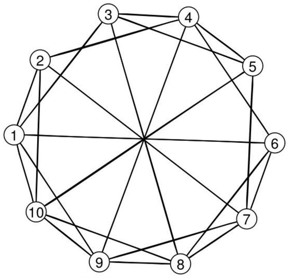
[0102] Step 1. Propose an original optimization problem model (1) for a multi-intelligent system with both local set constraints and local equality constraints;
[0103] Step 2, the original optimization problem model (1) obtained in step 1 is converted into a convex optimization problem model (2) that is convenient for distribution processing;
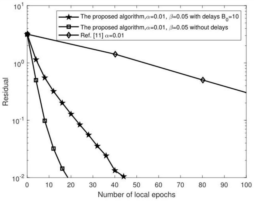
[0104] Step 3. Propose a distributed projection algorithm based on variance reduction technology (3) to solve the constrained convex optimization problem model (2), that is, use local stochastic average gradient to unbiasedly estimate the local full gradient, so as to reduce the problem in each iteration The heavy computational burden caused by calculating the full gradient of all local objective functions in ;...
PUM
 Abstract
Description
Claims
Application Information
 - R&D
- Intellectual Property
- Life Sciences
- Materials
- Tech Scout
- Unparalleled Data Quality
- Higher Quality Content
- 60% Fewer Hallucinations
Browse by: Latest US Patents, China's latest patents, Technical Efficacy Thesaurus, Application Domain, Technology Topic, Popular Technical Reports.
© 2025 PatSnap. All rights reserved.Legal|Privacy policy|Modern Slavery Act Transparency Statement|Sitemap|About US| Contact US: help@patsnap.com