Reverse time migration method and device based on finite element
A technology of reverse time migration and finite element, applied in the direction of measuring devices, seismology, instruments, etc., can solve problems such as large amount of calculation, low parallel efficiency, staying in two-dimensional model experimental research, etc., to achieve high precision and improve efficiency Effect
- Summary
- Abstract
- Description
- Claims
- Application Information
AI Technical Summary
Problems solved by technology
Method used
Image

Examples
Embodiment Construction
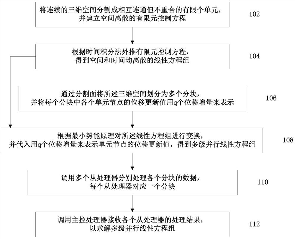
[0129] Preferred embodiments of the present application will be described in more detail below with reference to the accompanying drawings. Although preferred embodiments of the present application are shown in the drawings, it should be understood that the present application may be embodied in various forms and should not be limited to the embodiments set forth herein. Rather, these embodiments are provided so that this application will be thorough and complete, and will fully convey the scope of this application to those skilled in the art.
[0130] See figure 1 . figure 1 A flowchart showing a method for establishing a prestack time migration velocity field according to an embodiment of the present application. As shown in the figure, the method includes the following steps.
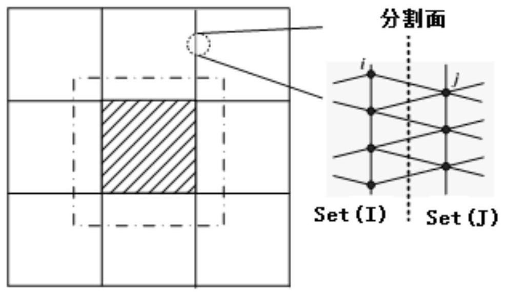
[0131] In step 102, the continuous three-dimensional space is divided into a finite number of interconnected but non-overlapping units, and a spatially discrete finite element governing equation i...
PUM
 Abstract
Description
Claims
Application Information
 - R&D
- Intellectual Property
- Life Sciences
- Materials
- Tech Scout
- Unparalleled Data Quality
- Higher Quality Content
- 60% Fewer Hallucinations
Browse by: Latest US Patents, China's latest patents, Technical Efficacy Thesaurus, Application Domain, Technology Topic, Popular Technical Reports.
© 2025 PatSnap. All rights reserved.Legal|Privacy policy|Modern Slavery Act Transparency Statement|Sitemap|About US| Contact US: help@patsnap.com