Variable support robust transform for multiple description coding
a multi-description coding and variable support technology, applied in the field of encoding and decoding of temporally coherent data, can solve the problems of insufficient protection of error correction/channel coding at low bit cost, retransmission introduce delay, interpolation recovery techniques recover missing data from available surrounding data,
- Summary
- Abstract
- Description
- Claims
- Application Information
AI Technical Summary
Benefits of technology
Problems solved by technology
Method used
Image
Examples
case 1
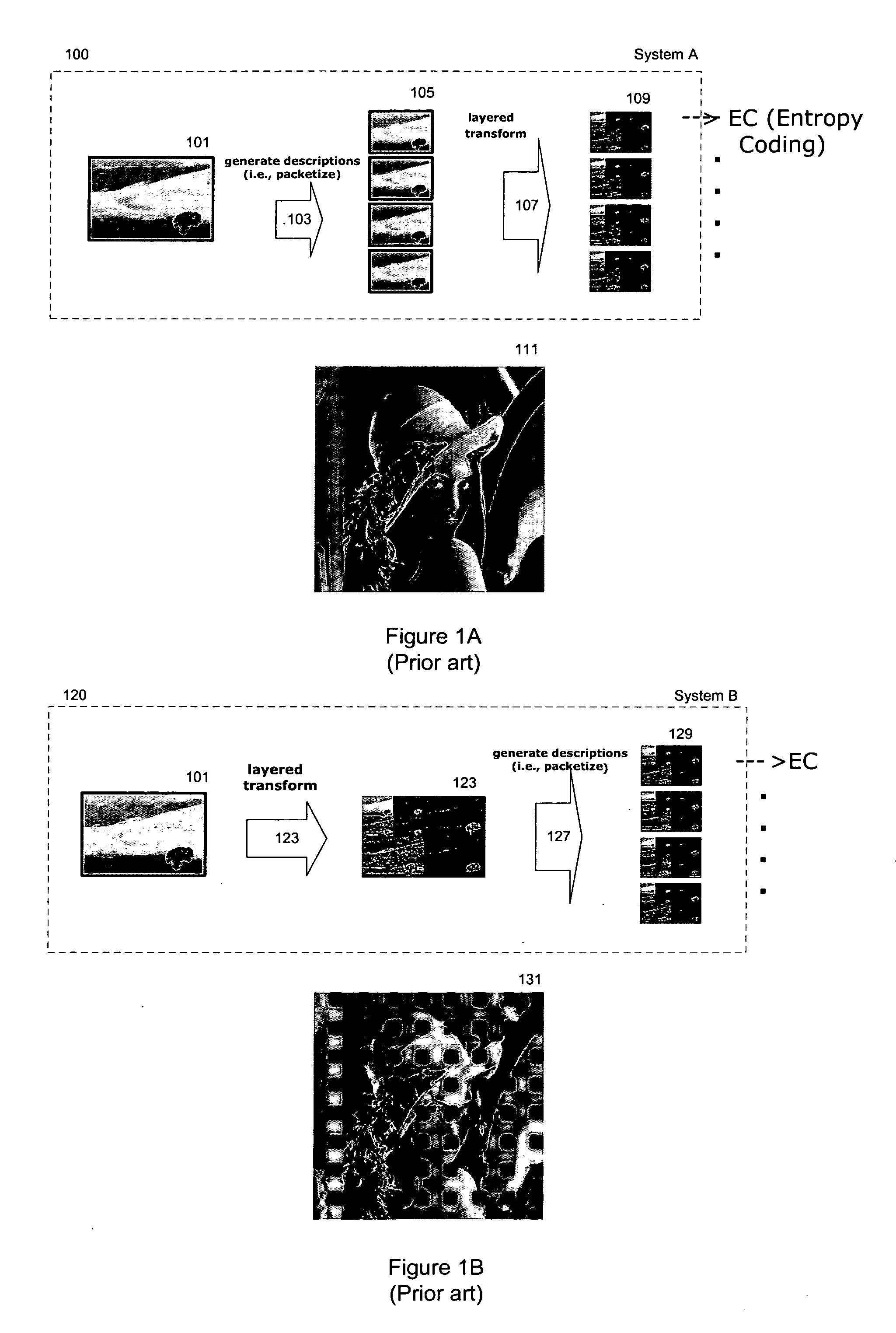
[0059] Case 1 involves a prediction point that skips over three descriptions, i.e., jc= . . . −8,−4,0,4,8, . . . . The update involves an average of points four pixels / descriptions apart. The filter matrix A is illustrated in Table 1. Because the support of the filters are completely contained within single description, this system exhibits good robustness but poor compression. This is case is referred to as System A.
TABLE 1k =−8−7−6−5−4−3−2−101234567−40.50.5−31−20.50.5−11i = 00.50.51120.50.531
case 2
[0060] Case 2 is update and prediction done on neighboring data, i.e., jc= . . . −2,−1,0,1,2, . . . (prediction involves every point), and matrix A has the form shown in Table 2. This system involves prediction and update filters that spread across description boundaries, and thus has good compression, but strong error propagation. This case is referred to as system B.
TABLE 2k =−8−7−6−5−4−3−2−101234567−40.50.5−31−20.50.5−11i = 00.50.51120.50.531
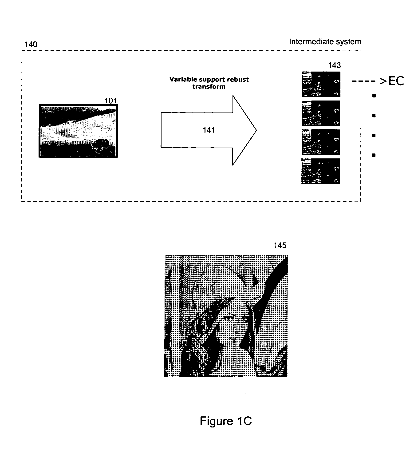
[0061] In case 3, referred to as System C, jc= . . . −4,−2,0,2,4 . . . so prediction is done using every other description (i.e., skip one description), and the update / low pass spreads across descriptions (but skips one description) with equal weight. The matrix A has the form shown in Table 3. This is an intermediate system falling between Systems A and B in the compression-robustness characterization space.
TABLE 3k =−8−7−6−5−4−3−2−101234567−4.5.5−31−2.5.5−11i = 0.5.5112.5.531
case 4
[0062] Case 4, also referred to as System D, has jc= . . . −2,−1,0,1,2 . . . so that prediction is done across descriptions (every description included), and the update spreads across descriptions (but skips one description). The matrix A has the form shown in Table 4. For intermediate systems, the prediction and update must be more carefully tuned to each other. In this example, the unequal weights 0.75 / 0.25 are used to spread out the low pass data points more evenly and yield a more symmetric prediction filter (but not linear phase).
TABLE 4k =−8−7−6−5−4−3−2−101234567−4.75.25−31−2.25.75−11i = 0.75.25112.25.7531
PUM
 Abstract
Description
Claims
Application Information