

Method, apparatus, and computer program product for optimizing parameterized models using functional paradigm of spreadsheet software
a spreadsheet software and functional paradigm technology, applied in the field of methods, apparatuses, and computer program products for optimizing parameterized models using the functional paradigm of spreadsheet software, can solve the problems of constrained optimization involving systems of differential and differential equations that are beyond the limitations of existing add-ins, prior art add-ins do not offer an integrated solution to this class of problems, and solvers for differential equations in excel have been rather limited
- Summary
- Abstract
- Description
- Claims
- Application Information
AI Technical Summary
Benefits of technology
Problems solved by technology
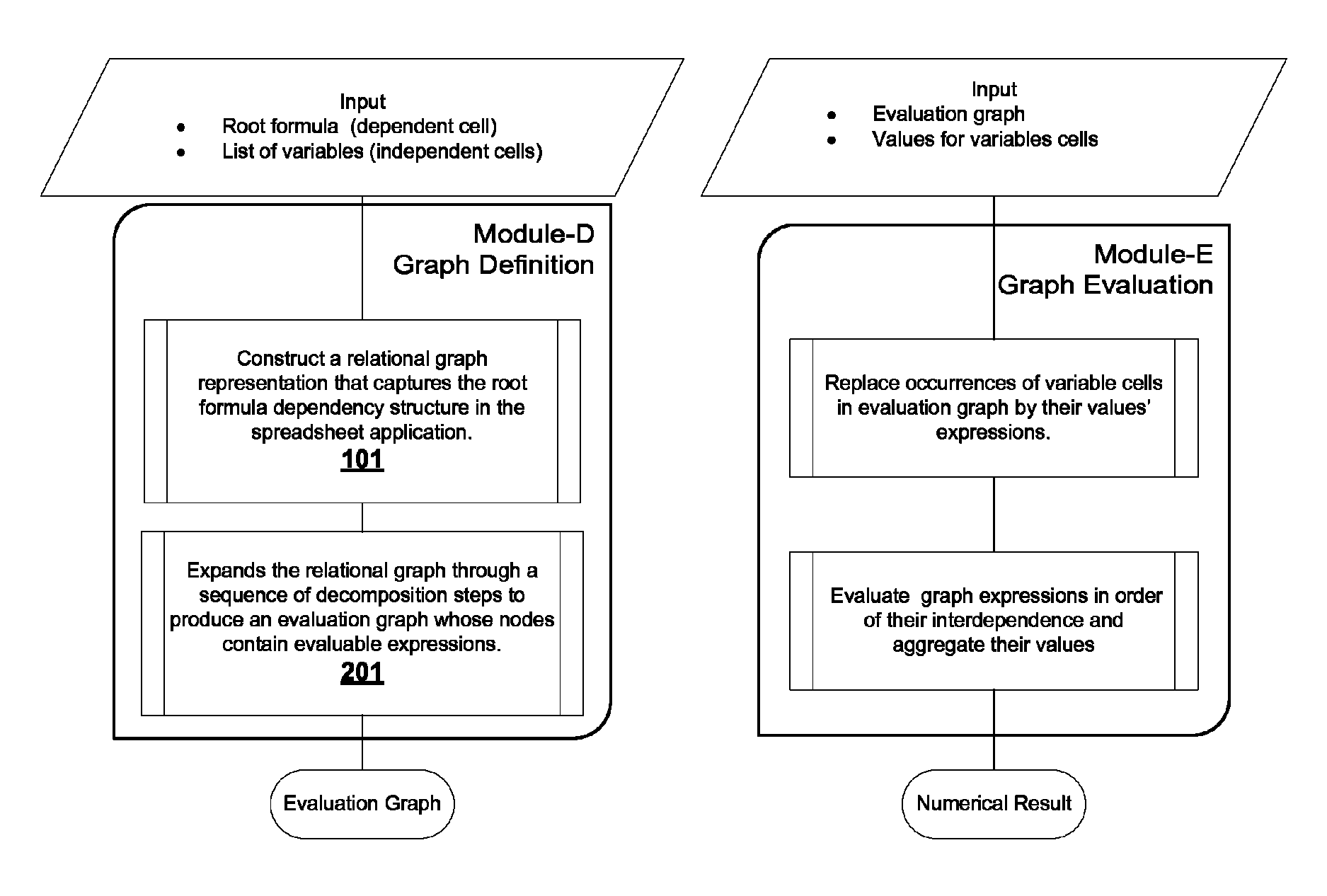
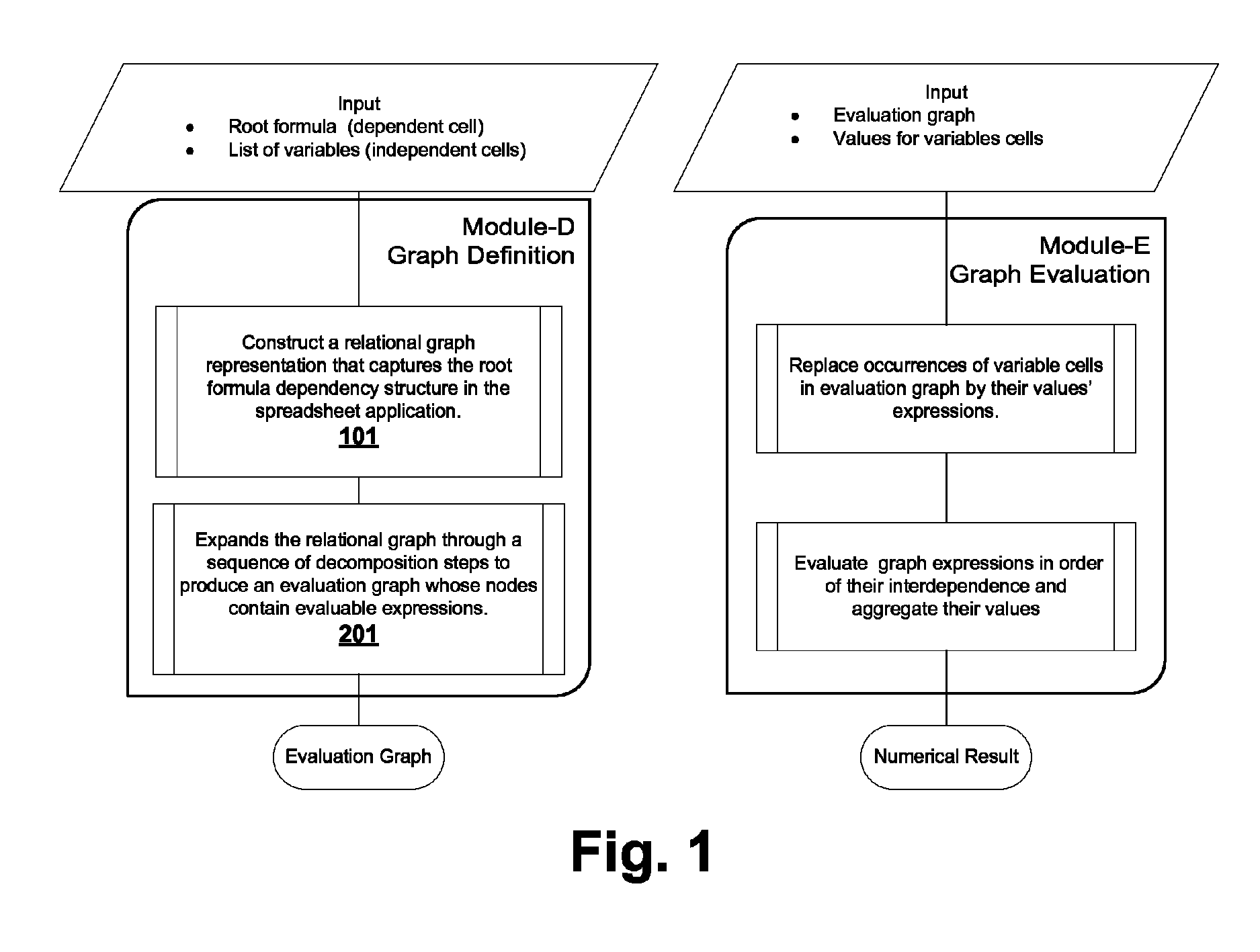
Method used
Image

Examples
example 1
Customizing a 2nd Order Dynamical System Response
[0249]Consider the 2nd order differential equation
[0250]ⅆ2xⅆt2+2ζwnⅆxⅆt+wn2x=0
which describes a dynamical system with inertia, energy storage, and dissipation components. In this formulation, x(t) represents the displacement, wn represents the natural frequency, and ζ the damping ratio. The objective is to find optimal values for wn and ζ such that the system has an absolute overshoot value of 2.0 at a peak time of 2.0 seconds, in response to an initial displacement condition of one. The overshoot is defined as the maximum absolute peak value of the displacement curve x(t), and the peak time is the time at which the overshoot is attained.
Step 1: Solve the differential system with initial values for the design parameters.
[0251]In order to use IVSOLVE( ), the 2nd order system is represented as two first order differential equations:
[0252]ⅆxⅆt=vⅆvⅆt=-2ζwnv-wn2x
[0253]The problem input definition for IVSOLVE( ) is shown in Table...
example 2
Computing Train Propulsion and Travel Time
[0261]A frictionless train uses a constant propulsion force to accelerate, but relies solely on the gravitational pull of the Earth, as well as aerodynamic drag for deceleration. Based on the assumptions of Table 21, we need to compute the required propulsion force and the trip time for the train to travel between two cities 1000 km apart through a straight tunnel.
[0262]
TABLE 21Train massm = 100,000 (kg)Distance travelledd = 1000,000 (m)Earth radiusRe = 6371,000 (m)Gravitational constantg = 10 m / s2Propulsion forceFp = constant (N) Unknown valueDrag forceFd(v) = 0.5 * v2(N)Gravitational forceFg(θ) = m * g * cos (θ) (N)
Constrained Optimization Model
[0263]The forces acting on the train during its motion between the two cities are depicted in FIG. 12. Applying Newton's second law, the motion for the train is governed by the 2nd order differential equation:
m*{umlaut over (x)}=Fp−Fd({dot over (x)})+Fg(θ(x))
with initial conditions x(0)=0, {dot over...
PUM
 Abstract
Description
Claims
Application Information