Method for judging self-given delay repeatability of streaming data in real time
A data stream and data element technology, which is applied in the direction of electrical digital data processing, special data processing applications, digital data information retrieval, etc.
- Summary
- Abstract
- Description
- Claims
- Application Information
AI Technical Summary
Problems solved by technology
Method used
Image

Examples
Embodiment Construction
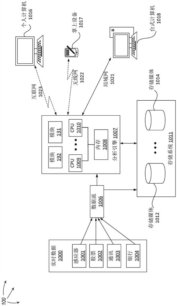
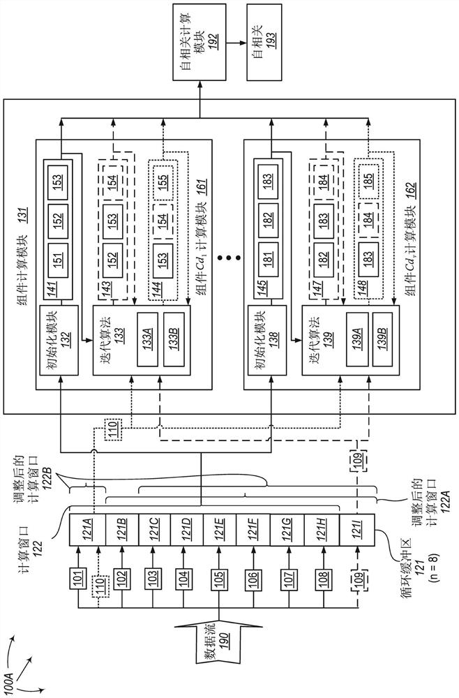
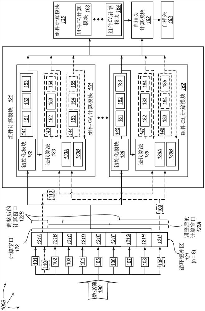
[0038]Computing autocorrelation is an effective way to judge the repeatability of time series or streaming big data itself for a given delay. The present invention extends to a method for judging the repeatability of the given delay of the stream data itself in real time by iterating the autocorrelation of the specified delay l (1≤l1) of the stream data , System and Computing Device Program Products. A computing system consists of one or more processor-based computing devices. Each computing device contains one or more processors. The computing system includes an input buffer. This input buffer holds large data or streaming data elements. This buffer can be in memory or other computer-readable media, such as hard disk or other media, or even multiple distributed files allocated on multiple computing devices, which are logically interconnected end-to-end to form a "circular buffer" ". Multiple data elements from the data stream that are involved in autocorrelation calculat...
PUM
 Abstract
Description
Claims
Application Information