Iron loss calculation method based on local hysteresis loop model
A technology of hysteresis loop and calculation method, applied in complex mathematical operations, design optimization/simulation, etc., can solve the problems of inaccurate hysteresis loss and partial hysteresis loop not closing, and achieve the effect of accurate core loss
- Summary
- Abstract
- Description
- Claims
- Application Information
AI Technical Summary
Problems solved by technology
Method used
Image

Examples
specific Embodiment approach 1
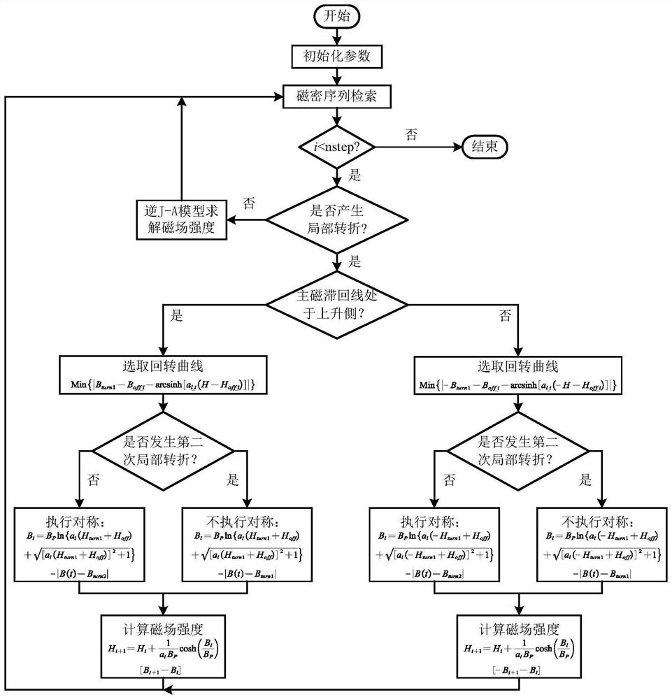
[0035] Specific implementation mode one: combine figure 1 Describe this embodiment, this embodiment is an iron loss calculation method based on a local hysteresis loop model, including the following steps:
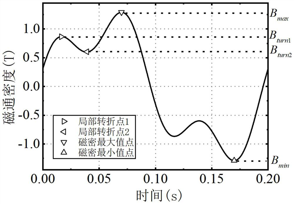
[0036] Step 1. Obtain the magnetic flux density sequence of the silicon steel sheet and the hysteresis loop data. The hysteresis loop includes a main hysteresis loop and a gyration curve, and the main hysteresis loop includes n magnetic flux densities;
[0037] Step 2. Judging whether the i-th magnetic flux density on the main hysteresis loop has a local turning point, wherein, the initial value of i is 1, i=1,2,...,n, if no local turning point occurs, then Use the inverse J-A model to calculate the magnetic field intensity corresponding to the i-th magnetic flux density, and re-retrieve the magnetic flux density sequence until a local turning point occurs, record the point when the local turning point occurs as the first local turning point, and the first local If the tu...
specific Embodiment approach 2
[0062] Embodiment 2: The difference between this embodiment and Embodiment 1 is that the inverse J-A model in the step 2 is:
[0063]
[0064] In the formula, t is the time of the previous step; Δt is the time change from the previous step to the current step; B is the magnetic flux density, H is the magnetic field intensity, and the magnetic flux density B is known and given in the form of time series; B(t) is the magnetic flux density of the previous step, B(t+Δt) is the magnetic flux density of the current step, ΔB is the change of the magnetic flux density from the previous step to the current step, H(t) is the magnetic field intensity of the previous step; H(t +Δt) is the magnetic field strength of the current step, M is the magnetization strength, H e , B e is the effective magnetic field strength and effective magnetic flux density, M an is the ideal magnetization fitted by the Langevin equation, M irr is the reversible magnetization, a, α, c, k, M s are the five...
specific Embodiment approach 3
[0067] Specific embodiment three: the difference between this embodiment and specific embodiment one or two is that the direction coefficient δ is:
[0068]
[0069] Other steps are the same as those in Embodiment 1 or 2.
PUM
 Abstract
Description
Claims
Application Information