Noise detection for audio encoding

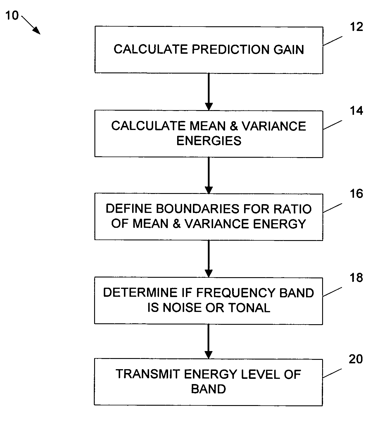
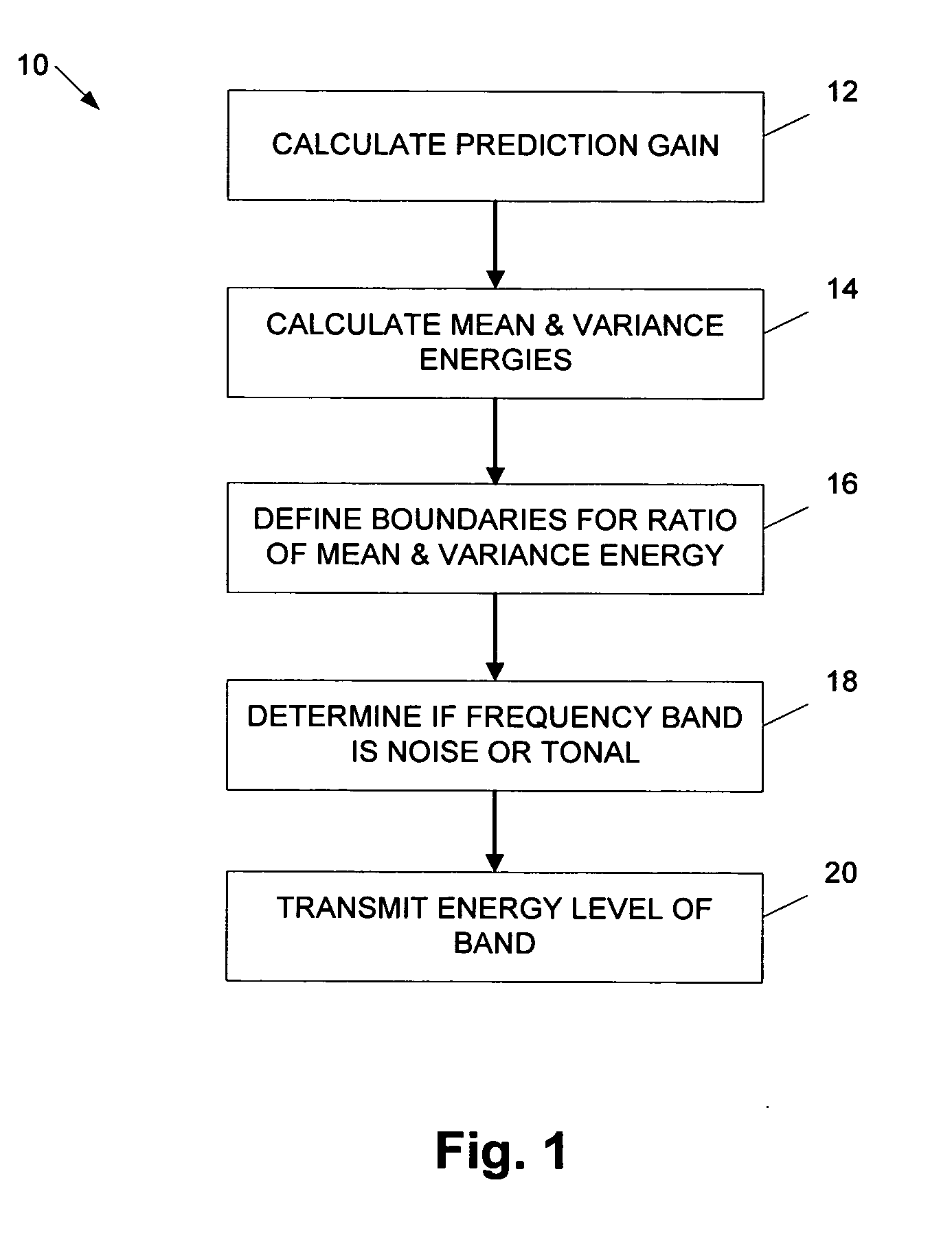
[0020]FIG. 1 illustrates a flow diagram 10 depicting operations performed in the estimation and detection of noise and noise-like spectral signal segments in audio coding. Additional, fewer, or different operations may be performed depending on the embodiment. In an operation 12, a gain prediction for the spectral samples corresponding to each frequency band is calculated. In this calculation, the variable x represents a frequency domain signal of length N: x=F(xt) where xt is the time domain input signal and F( ) denotes time-to-frequency transformation. The variable sfbOffset of length M represents the boundaries of the frequency bands, which follow also the boundaries of the critical bands of human auditory system.

[0021] A gain prediction is calculated for each frequency band. In an exemplary embodiment, the prediction gain is determined by applying linear predictive coding (LPC) principles to spectral samples within each frequency band and accumulating the resulted gain across the frequency bands to obtain an average prediction gain aGain for the current frame as: aGain = 1 M · ∑ i = 0 M - 1 ⁢ sbGain ⁡ ( i ) sbGain ⁡ ( i ) = { fGain i , gThr , ⁢ fGain i gThr otherwise

where fGaini is the prediction gain of the ith frequency band and gThr is the global threshold for the prediction gain. This threshold prevents the average prediction gain from being too high in case some of the spectral bands have significant prediction gain. In an example implementation, the value of gThr is set to 1.45.

[0022] The prediction gain for the ith frequency band can be obtained by solving the normal equations: ∑ k = 1 P ⁢ a k · R i ⁡ ( n - k ) = R i ⁡ ( n ) , 1 ≤ n ≤ P

where P defines the order of the filter coefficients ak and R is the autocorrelation sequence of the spectral samples calculated by: R i ⁡ ( n ) = ∑ k = 1 sfbLen - 1 ⁢ x ⁡ ( sfbOffset ⁡ ( i ) + k ) · x ⁡ ( sfbOffset ⁡ ( i ) + k - n )

where sfbLen=sfbOffset(i+1)−sfbOffset(i) is the length of the ith frequency band.

[0023] The predictor order P can be determined based on the length of the frequency band:

p=min(10, sfbLen/4

One solution of the normal equations is performed by the Levinson-Durbin recursion. The following operations can be performed for m=1, . . . , P, where ak(m) denotes the kth coefficient of an mth order predictor by: akk m = ⁢ R i ⁡ ( m ) - ∑ k = 1 m - 1 ⁢ a k ( m - 1 ) · R i ⁡ ( m - k ) E m - 1 i a m ( m ) = ⁢ akk m a k ( m ) = ⁢ a k ( m - 1 ) - akk m · a m - k ( m - 1 ) , 1 ≤ k ≤ m - 1 E m i = ⁢ ( 1 - akk m 2 ) · E m - 1 i where ⁢ ⁢ E 0 i = ⁢ R i ⁡ ( 0 ) .

[0024] The prediction gain can be obtained by: fGain i = R i ⁡ ( 0 ) E P i

Next, mean and variance energies can be calculated for each frequency band by: eMean i = 1 sfbLen · ∑ k = 0 sfbLen - 1 ⁢ x ⁡ ( sfbOffset ⁡ ( i ) + k ) 2 eVar i = 1 sfbLen · ∑ k = 0 sfbLen - 1 ⁢ eMean i - x ⁡ ( sfbOffset ⁡ ( i ) + k ) 2

The mean and variance energies are used to define the boundaries for the ratio of the mean and variance energy and how much that ratio is allowed to vary in each frequency band. This range can be used to differentiate whether the frequency band is noise-like or tonal-like. The allowed range can be obtained by: eRatio = 1 M · ∑ i = 0 M - 1 ⁢ eMean i eVar i vMax = { eRatio , eRatio ≥ 1.0 1.0 ⁢ / ⁢ eRatio , otherwise ⁢ ⁢ acc = { 2.6 · aGain , 2.6 · aGain vThr vThr , otherwise ⁢ ⁢ eMeanMax = vMax acc ⁢ ⁢ eMeanMin = 1.0 ⁢ / ⁢ eMeanMax

where vThr defines the threshold for the mean energy range calculation. In the an example implementation, this value is set to 3.3, but also other values may be applied.

[0025] A stage of decisions can be made for each frequency band to see whether the band is noise/noise-like or tonal/tonal-like as follows isNoise i 1 = { 1 , fGain i w i 1 · aGain · pGain i 0 , otherwise

where pGaini is the adjusted prediction gain of previous frame for the ith frequency band and wi1 is the frequency band dependent weighting factor, which is updated according to:

wi1=√{square root over (wi−11)}

where w−11=0.7 in an example implementation. Also, isNoise i 2 = { 1 , isNoise i 1 ⁢ == ⁢ 1 ⁢ ⁢ and ⁢ ⁢ eComp i w i 2 · cThr 0 , otherwise

where eCompi defines the energy compression ratio of the ith frequency band, wi2 is frequency band dependent weighting factor, and cThr is global threshold value for the energy compression ratio. In the current implementation the value of cThr is set to 10−0.1. The energy compression ratio can be calculated according to: y i ⁡ ( n ) = e ⁡ ( n ) · ∑ k = 0 sfbLen - 1 ⁢ x ⁡ ( sfbOffset ⁡ ( i ) + k ) · cos ⁡ ( ( 2 · k + 1 ) · n · π ) 2 · sfbLen , ⁢ 0 ≤ n ≤ sfbLen - 1 e ⁡ ( n ) = { 2 - 1 , n ⁢ ⁢ == ⁢ 0 1 , otherwise ⁢ ⁢ eComp i = ∑ k = 0 sfbLen ⁢ / ⁢ 2 - 1 ⁢ y i ⁡ ( k ) 2 ∑ k = sfbLen ⁢ / ⁢ 2 sfbLen - 1 ⁢ y i ⁡ ( k ) 2

The frequency dependent weighting factor wi2 can be updated according to:

wi2=√{square root over (wi−12)}

where w−12=0.7 in an example implementation. The noise decision stage is: isNoise i 3 = { 1 , isNoise i 2 == 1 ⁢ ⁢ and ( eMVRatio i eMeanMax or eMVRatio i eMeanMin ) 0 , otherwise eMVRatio i = eMean i eVar i

If the ith frequency band was assigned to be noise or noise-like, i.e., isNoisei3=1, then what is transmitted to the receiver is the energy level of the band. The same signaling method used in an AAC codec can be used here. The prediction gain related to the time dimension of each frequency band is finally updated as: pGain i = { 0.25 · pGain i + 0.75 · fGain i , pGain i != 1.0 ⁢ ⁢ and ⁢ ⁢ isNoise i 3 == 1 fGain i , pGain i == 1.0 ⁢ ⁢ and ⁢ ⁢ isNoise i 3 == 1 1.0 , otherwise

Equation (13) may be realized with fast algorithms that use transform length of 2n. In case the length of the frequency band does not fit into these conditions, that is, the length is smaller than the length of the transform, zero padding can be used. Also, it is known that human auditory system is more sensitive at low frequencies than at high frequencies. Therefore, for optimal performance, it is advantageous to limit the lowest possible noise frequency band to some threshold frequency, such as 5 kHz, but also other values are applicable.

[0026] In an implementation using an AAC encoder, the following parameters can be used. The time-to-frequency transformation F( ) is 128- or 1024-point MDCT, the sfbOffset table depends on the sampling rate and are listed in the AAC specifications but, for example, at 44 kHz the table for 128- and 1024-point MDCTs are as: [0027] M=49; [0028] sfbOffset—1024[]={0, 4, 8, 12, 16, 20, 24, 28, 32, 36, 40, 48, 56, 64, 72, 80, 88, 96, 108, 120, 132, 144, 160, 176, 196, 216, 240, 264, 292, 320, 352, 384, 416, 448, 480, 512, 544, 576, 608, 640, 672, 704, 736, 768, 800, 832, 864, 896, 928, 1024}; [0029] M=14; [0030] sfbOffset—128[]={0, 4, 8, 12, 16, 20, 28, 36, 44, 56, 68, 80, 96, 112, 128};

If the start of noise detection band is limited to 5 kHz, the tables are as: [0031] M=22; [0032] sfbOffset—1024[]={264, 292, 320, 352, 384, 416, 448, 480, 512, 544, 576, 608, 640, 672, 704, 736, 768, 800, 832, 864, 896, 928, 1024}; [0033] M=6; [0034] sfbOffset—128[]={44, 56, 68, 80, 96, 112, 128};

[0035] It is also possible to define the start of noise detection band to be below 5 kHz. In this case it is advantageous to make the noise detection calculations separately; one set of calculations for the frequency bands below 5 kHz and the other set of calculations for frequency bands above 5 kHz. Also the thresholds related to prediction gain and mean energy threshold calculations can be adjusted to better cope with the sensitivity of human auditory system at low frequencies; values 1.15 and 4.0, respectively, provide best performance for the frequencies below 5 kHz.

[0036] The techniques described require no buffering of previous frame samples, which is one of the main drawbacks of prior solutions. Buffering typically extends to at least 2-3 past frames and with larger frame sizes this requires a lot of static RAM storage during encoding. The noise estimation is done using signal adaptive threshold values and no hard threshold levels are used which is typically used in prediction based noise estimation solutions. Furthermore, the complexity of the method plays no significant role in the whole encoder implementation as only few calculations are done for each frame and additional calculations are done only to those frequency bands which have high probability to be noise or noise-like. For example, the number of noise or noise-like frequency bands with respect to total number of frequency bands present can be less than half or more.

[0037] Simulations using the described techniques have shown that reliable noise detection can be achieved without introducing any perceptual distortions to the coded signals. The bitrate limit for the lowest possible bitrate depends on the signal content but, with typical signals, bitrate reduction between 5-15% can be expected when compared to an encoding where noise detection and substitution is not applied.

[0038]FIG. 2 illustrates a system 50 including the noise detection feature described herein. The exemplary embodiments described herein can be applied to any system capable coding of signals. An exemplary system 50 includes a terminal equipment (TE) device 52, an access point (AP) 54, a server 56, and a network 58. The TE device 52 can include memory (MEM), a central processing unit (CPU), a user interface (UI), and an input-output interface (I/O). The memory can include non-volatile memory for storing applications that control the CPU and random access memory for data processing. The I/O interface may include a network interface card of a wireless local area network, such as one of the cards based on the IEEE 802.1 1 standards.

[0039] The TE device 52 may be connected to the network 58 (e.g., a local area network (LAN), the Internet, a phone network) via the access point 54 and further to the server 56. The TE device 52 may also communicate directly with the server 56, for instance using a cable, infrared, or a data transmission at radio frequencies. The server 56 may provide various processing functions for the TE device 52.

[0040] The TE device 52 can be any electronic device, for example a personal digital assistant (PDA) device, remote controller or a combination of an earpiece and a microphone. The TE device 52 can be a supplementary device used by a computer or a mobile station, in which case the data transmission to the server 56 can be arranged via a computer or a mobile station. The TE device 52 can be a personal computer (PC) or other computing device in which, for example, music is encoded and sent over an air channel to a mobile device or over the Internet to another PC. In an exemplary embodiment, the TE device 52 is a mobile station communicating with a public land mobile network, to which also the server 56 is functionally connected. The TE device 52 connected to the network 58 includes mobile station functionality for communicating with the network 58 wirelessly. The network 18 can be any known wireless or wired network, for instance a network supporting the GSM service, a network supporting the GPRS (General Packet Radio Service), or a third generation mobile network, such the UMTS (Universal Mobile Telecommunications System) network according to the 3GPP (3rd Generation Partnership Project) standard. The functionality of the server 56 can also be implemented in the mobile network. The TE device 56 can be a mobile phone used for speaking only, or it can also contain PDA (Personal Digital Assistant) functionality.

[0041] While several embodiments of the invention have been described, it is to be understood that modifications and changes will occur to those skilled in the art to which the invention pertains. The invention is not limited to a particular embodiment, but extends to various modifications, combinations, and permutations that nevertheless fall within the scope and spirit of the appended claims.