Non-perspective variable-scale map displays
a variable-scale, map-based technology, applied in the field of digital images, can solve the problems of computational problems associated with points that fall near or behind, and the view of angled perspectives is limited in how it depicts
- Summary
- Abstract
- Description
- Claims
- Application Information
AI Technical Summary
Benefits of technology
Problems solved by technology
Method used
Image
Examples
example 1
The “Exponential” Variable-scale Map
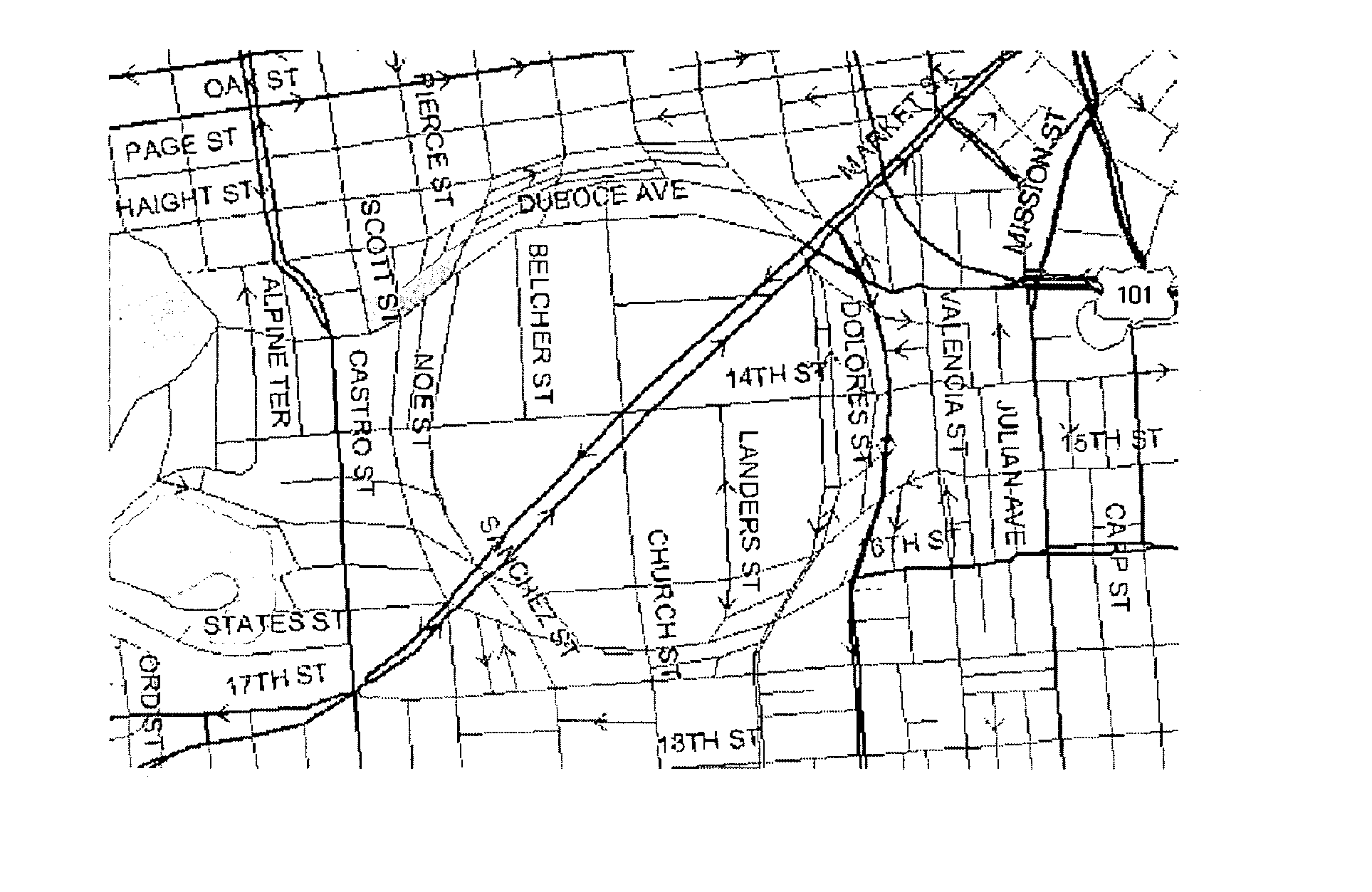
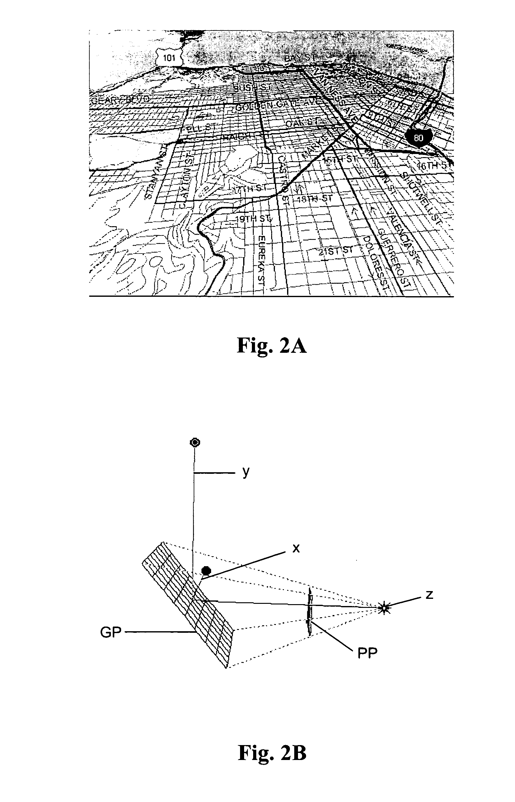
[0047] The “Exponential” View as formulated by equations (7) below, has been found to have useful display characteristics, especially if a horizon is desired.
{overscore (y)}=k(1−eλy). F(x,y)=xƒ({overscore (y)}) G(x,y)={overscore (y)}g(X) (7)
where λ and k are suitable constants.
[0048] Again, assume the x axis is the bottom of the map display. In the Exponential View, y is a function of y, where y is in the exponent of e. If 0<λ<1, then for large y the exponent approaches zero and what is left is a horizon, M, where M=k. The coefficient λ controls the speed at which the y axis is compressed and k sets the height of the horizon on the display. A straight line or a concave shape can be used to define ƒ({overscore (y)}) as was described earlier.
example 2
The “Power” Variable-scale Map. The Power View as formulated in (8) below, also has useful display characteristics, especially if no horizon is desired.
[0049]
{overscore (y)}=(αy+k)λ−kλ,
F(x,y)=xƒ({overscore (y)}),
G(x,y)={overscore (y)}g(X), (8)
where α, λ, and k are suitable constants.
[0050] As before, assume the x axis is the bottom of the map display. In the Power View, {overscore (y)} is a function of y raised to a power, λ,. Take 0λ has slope 1, k=λ80 / (1−λ). The constant α will then have a stretching or shrinking effect.
[0051] The power function has no horizon (the y values have no upper limit) except to the extent that the map itself has a limit or the designer imposes a limit. Because there is no horizon there is no vanishing point. The shape of the vertical lines can thus be defined as f(y_)=bb+y_.(9)
[0052] If the map is assumed to be bounded by {overscore (y)}
example 3
The “Logarithmic” Variable-scale Map
[0054] The Logarithmic View is formulated in (10) below.
{overscore (y)}=λ log(αy+k)−log(k),
F(x,y)=xƒ({overscore (y)}),
G(x,y)={overscore (y)}g(X), (10)
where α, 80 , and k are suitable constants.
[0055] As before, assume the x axis is the bottom of the map display. In the logarithmic view, {overscore (y)} is a logarithmic function of y. Take 0<λ and k is chosen to be a point away from 0, typically near the point where the power function λlog({overscore (y)}) has slope 1, k=λ. The constant a will then have a stretching or shrinking effect.
[0056] Similar to the power function, the logarithmic function has no horizon (they values have no upper limit) except to the extent that the map itself has a limit or the designer imposes a limit. Because there is no horizon there is no vanishing point. The shape of the vertical lines can thus be defined as f(y_)=bb+y_.(11)
[0057] If the map is bounded by {overscore (y)}
PUM
 Abstract
Description
Claims
Application Information


