Robust testing for discrete-time and continuous-time system models
a system model and computer model technology, applied in the field of computer model verification, can solve the problems of affecting the safety of embedded devices, tedious process, and one of the tedious processes of model based design
- Summary
- Abstract
- Description
- Claims
- Application Information
AI Technical Summary
Problems solved by technology
Method used
Image
Examples
example 2
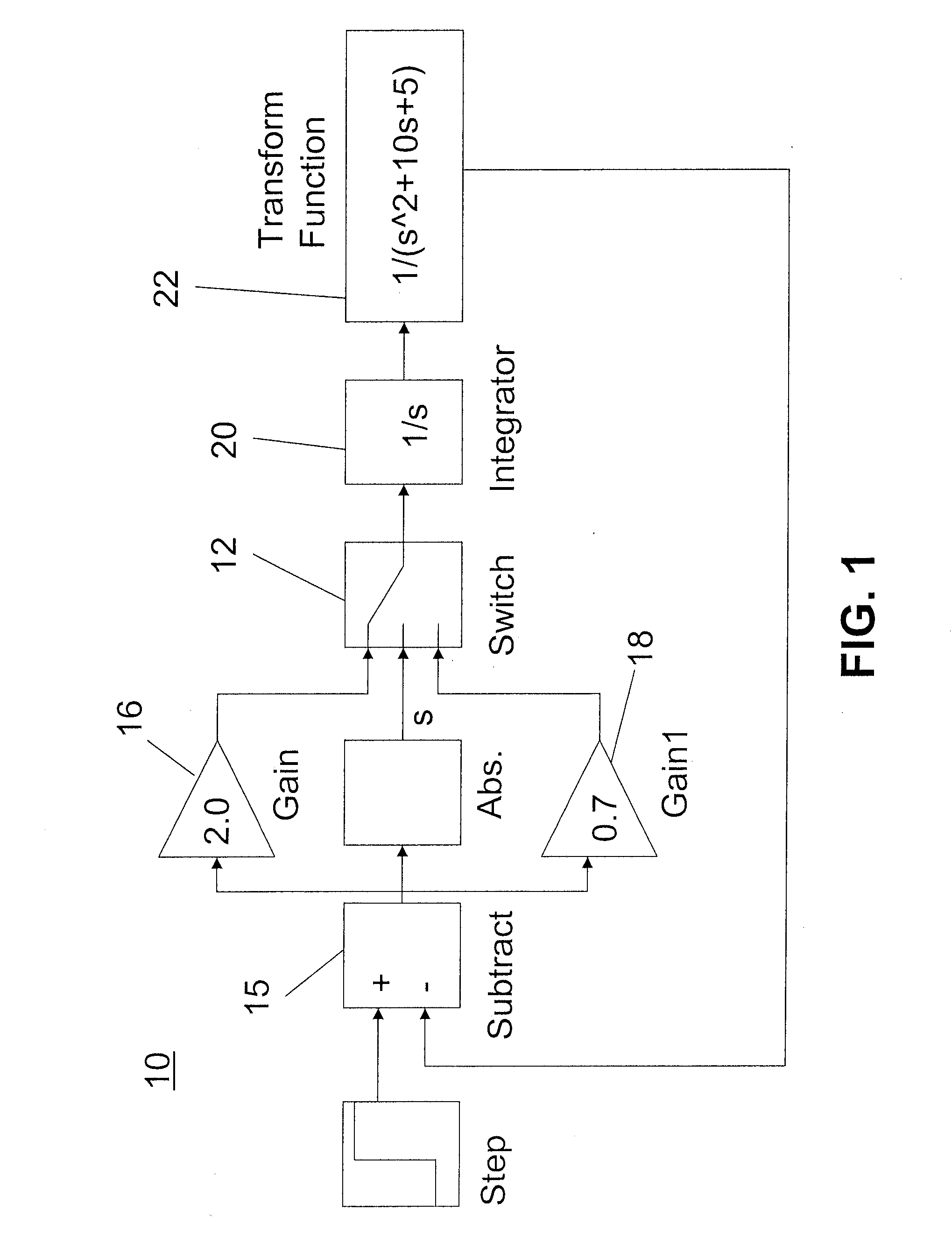
[0061]Consider the continuous-time model of FIG. 1 where a transfer function block 22 has been decomposed into a basic integrator 20, sum 15 and gain blocks 16, 18. The resulting system has 3 integrators and 6 gain blocks in total. The discretization of the system was performed with the Simulink™ model discretizer using zero-order hold (zoh) and a sample step of 0.1 sec. The robustness of the simulation is determined with initial conditions [−0.1, 0.1]3 and variation of %1 in the parameter values. The Simulink™ simulation is performed with initial conditions [0 0 0]T and the parameter values of Gain=2.0 (16) and Gain1=0.7 (18) as in FIG. 1. RobSimDt takes 31 sec to perform the guaranteed simulation and 5827 affine terms were generated. The result of the computation for the signal y detected 5 points where the simulation is non-robust. Below, we present how RobSimDt displays one of the warnings of possible non-robustness:
>> dispwarn (wd2, 5)Warning 5In the block ‘Switch’ at time 3.6T...
example 3
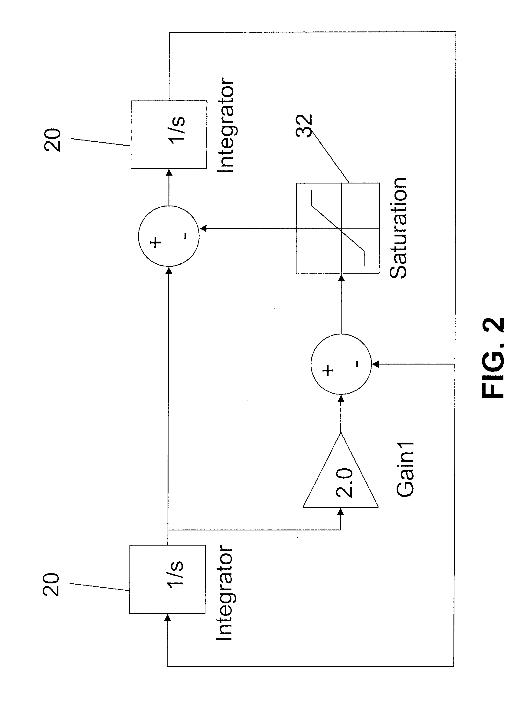
[0068]Consider the Simulink™ model in FIG. 2 which contains a non-linearity in the form of a saturation block 32. The saturation block 32 operates as follows. If the input signal is greater than an upper bound, then the output is set to the upper bound and if the input signal is lower than the lower bound, then the output of the block is set to the lower bound. In this example, the upper bound is set to 1 and the lower bound to −1. If we call the function “linmod” on the model of FIG. 2 at operating point [−1, 1]T then the system {dot over (x)}−A1x is derived which corresponds to the system dynamics without any saturation. However, if instead we use as operating point the value [−2, 1.6]T, which causes saturation to occur, “linmod” returns the system {dot over (x)}=A2x. A careful analysis of the system will reveal that the system dynamics at this operating point are affine and given by {dot over (x)}=A2x+b.
[0069]In order to circumvent the deficiencies of the “linmod” and related fun...
PUM
 Abstract
Description
Claims
Application Information