
Eureka
For R&D, Eureka makes reading and utilizing patents & technical documents easy.
Eureka AIR
Designed for self-driven R&D workflows. Generate viable solutions, solve complex R&D challenges, empower your innovation with AI.

Eureka Materials
Designed for material experts only. Revolutionize your material R&D, from search, analyze, to developing new materials.

TechResearch
Generate reliable direction feasibility study reports for your R&D in just a few steps.

TechSeek
Discover and master advanced knowledge NOW. Basics, ideas, possibilities, all at once.

TechMind
As an expert in R&D Theories, TechMind can generates customized viable solutions instantly.

TechRisk
Analyze your overall solution with one click, know your potential R&D risks in advance.

TechMonitor
Get weekly tech updates, stay abreast of the latest tech innovations and key insights.
System and method for optimizing passive control strategies of oscillatory instabilities in turbulent systems using finite-time lyapunov exponents
- Summary
- Abstract
- Description
- Claims
- Application Information
AI Technical Summary
Benefits of technology
Problems solved by technology
Method used
Image

Examples
example 1a
FTLE Field Computation in Thermoacoustic Instability Regime with CH* Chemiluminescence
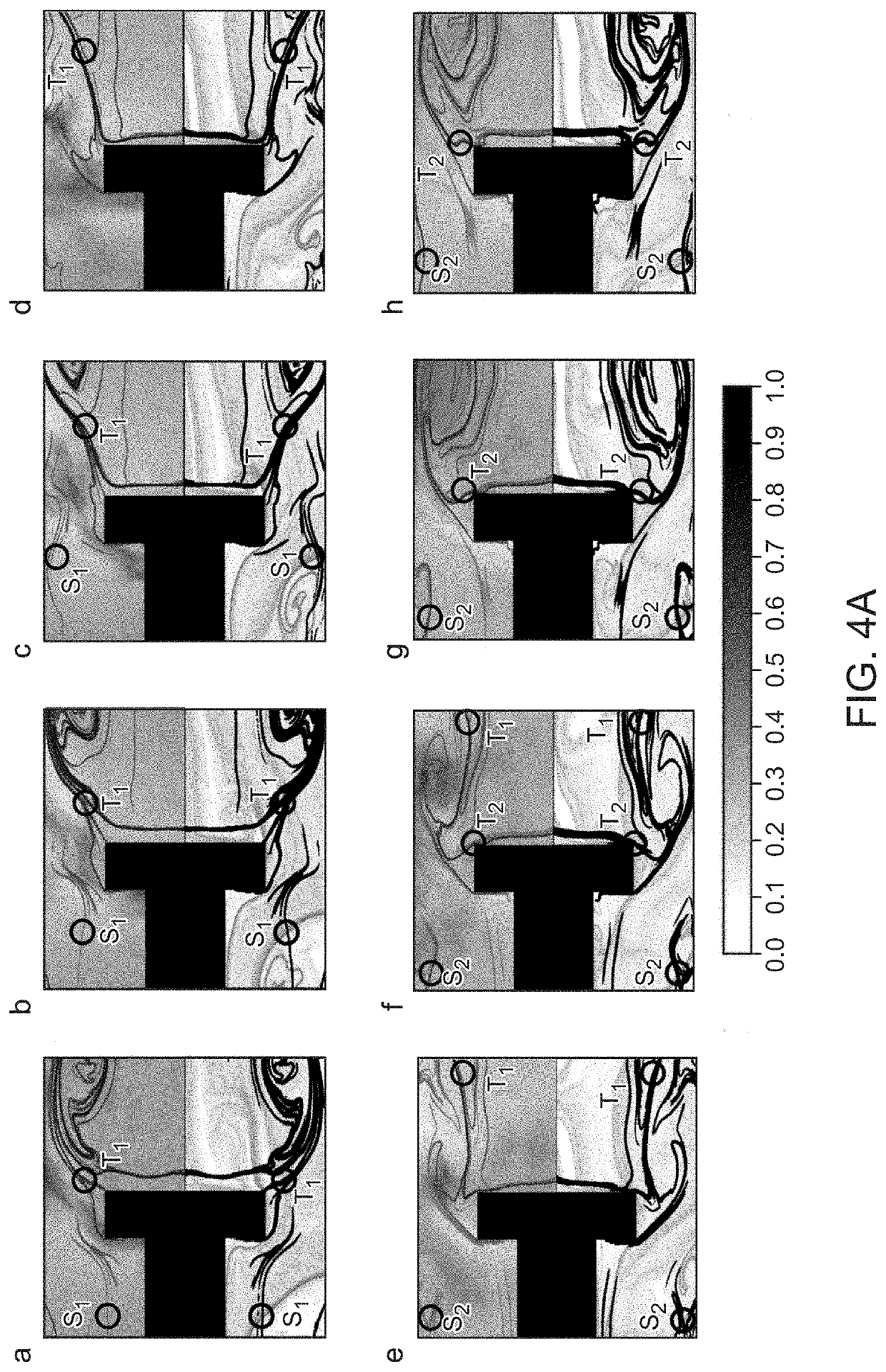
[0063]The ridges of FTLE fields computed with the velocity data along with CH* chemiluminescence showing local heat release rate fluctuations over a cycle of acoustic pressure oscillation in the regime of thermoacoustic instability is illustrated in FIG. 4A. The top panels (a) to (d) show backward-time FTLE ridges along with CH* chemiluminescence. In bottom panels (e) to (h), the ridges of backward-time FTLE field (black contour lines) are overlaid on ridges of forward-time FTLE field (gray filled contour). The contour levels have been normalized with the maximum value of the FTLE field. The critical regions are marked using black circles S1, S2, T1 and T2. Unsteady pressure fluctuations (p′) and global heat release rate fluctuations (q′) corresponding to a time period of thermoacoustic instability are shown in FIG. 4B. Flow is from left to right. The shear layer flapping in the upstream of the blu...
example 1b
FTLE Field Computation in Thermoacoustic Instability Regime with Vorticity Plots
[0064]Ridges of FTLE fields computed with the velocity data along with vorticity plots over a cycle of acoustic pressure oscillation in the regime of thermoacoustic instability is illustrated in FIG. 5A. The top panels (a) to (d) show vorticity plots. In bottom panels (e) to (h), the ridges of backward-time FTLE field (black contour lines) are overlaid on ridges of forward-time FTLE field (gray filled contour). The critical regions are marked using black circles S1, S2, T1 and T2 on both top and bottom panels. Unsteady pressure fluctuations (p′) and global heat release rate fluctuation (q′) corresponding to a time period of thermoacoustic instability are shown in FIG. 5B. Flow is from left to right.
example 2a
FTLE Field Computation in a Cycle of Burst Oscillation in the Intermittent Regime with CH* Chemiluminescence
[0065]Ridges of FTLE fields computed with the velocity data along with CH* chemiluminescence showing local heat release rate fluctuations over a cycle of burst oscillation in the intermittent regime is illustrated in FIG. 6A. The top panels (a) to (c) show backward-time FTLE ridges along with CH* chemiluminescence. In bottom panels (d) to (f), the ridges of backward-time FTLE field (black contour lines) are overlaid on ridges of forward-time FTLE field (gray filled contour). The contour levels have been normalized with the maximum value of the FTLE field. The critical regions are marked using black circles S1, S2, and T1. Unsteady pressure fluctuations (p′) and global heat release rate fluctuations (q′) corresponding to a time period of intermittency are shown in FIG. 6B. Flow is from left to right.
PUM
 Abstract
Description
Claims
Application Information
 - R&D Engineer
- R&D Manager
- IP Professional
- Industry Leading Data Capabilities
- Powerful AI technology
- Patent DNA Extraction
Browse by: Latest US Patents, China's latest patents, Technical Efficacy Thesaurus, Application Domain, Technology Topic, Popular Technical Reports.
© 2024 PatSnap. All rights reserved.Legal|Privacy policy|Modern Slavery Act Transparency Statement|Sitemap|About US| Contact US: help@patsnap.com