UUV (Unmanned Underwater Vehicle) path tracking method based on self-adaption sliding-mode control

An adaptive sliding mode and path tracking technology, applied in adaptive control, general control system, control/regulation system, etc., can solve the problems of complex construction and slow implementation, achieve high control accuracy, reduce chattering, Small chattering effect

Active Publication Date: 2017-01-04

HARBIN ENG UNIV

4 Cites 45 Cited by

AI-Extracted Technical Summary

Problems solved by technology

However, this method is complex to construct,...

the structure of the environmentally friendly knitted fabric provided by the present invention; figure 2 Flow chart of the yarn wrapping machine for environmentally friendly knitted fabrics and storage devices; image 3 Is the parameter map of the yarn covering machine

Abstract

The invention provides a UUV (Unmanned Underwater Vehicle) path tracking method based on self-adaption sliding-mode control. The method comprises the steps of 1, initializing; 2, obtaining a current state of a UUV; 3, establishing an underactuated UUV horizontal error equation to obtain the positional deviation xe, ye and a course deviation value psi e; 4, utilizing a sliding-mode control method to respectively design a speed sliding-mode control law, a position sliding-mode control law and a stem phase angle sliding-mode control law and enabling th ud to be zero, the xe to be zero and the psi e to be zero by controlling thrust Xprop, expected speed (shown in the following image) and torque Nprop; 5, updating a self-adaption law of handover gain and a self-adaption law of boundary layer thickness; 6, performing control input saturation compensation; 7, enabling k = k +1, returning to the step 2 and updating the control laws and the self-adaption laws for the next time to achieve the accurate control on the UUV horizontal path tracking. The UUV path tracking method can only depend on a controller which is designed according to a horizontal dynamical model to stabilize the system and is suitable for various underactuated UUVs.

Application Domain

Adaptive control

Technology Topic

Sliding mode controlSelf adaptive +6

Image

Examples

Experimental program(5)

Example Embodiment

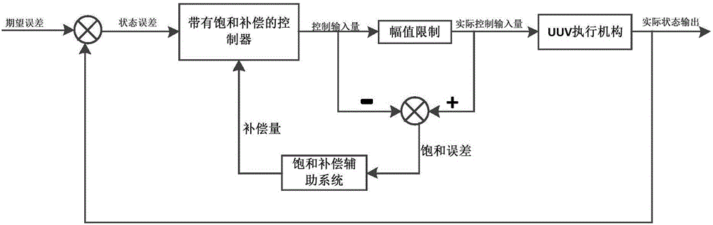
[0035] Specific implementation mode one: combine Figure 4 , the UUV path tracking method based on adaptive sliding mode of the present invention, comprises the steps:

[0036] Step 1. Initialization:

[0037] is various adaptive parameters k of UUV i ,λ i (i=1,2,3) assign initial value, and determine its ideal speed u for the path following process d , define update times t=0;

[0038] Step 2. Obtain the current state of the UUV:

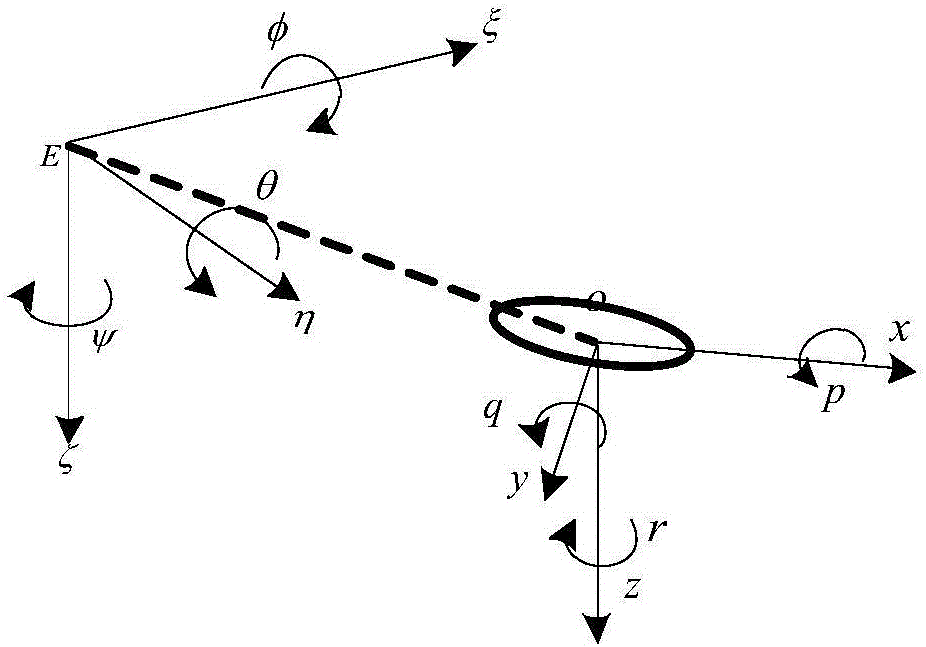
[0039] The current moment status is obtained through a series of sensors of the UUV itself: u, v are the longitudinal and lateral speeds (m/s), r are the yaw angular speeds (rad/s), and x, y are the UUV relative to the fixed coordinates position of the system (m), ψ is the yaw angle (rad), determine the longitudinal velocity error e u =u-u d;

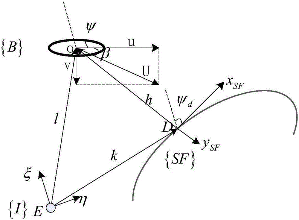
[0040] Step 3. Based on the Serret-Frenet coordinate system, establish the underactuated UUV horizontal plane error equation to obtain the position deviation x e ,y e and heading deviation ψ e;

[0041] Step 4. Use the sliding mode control method to design the speed sliding mode control law, the position sliding mode control law and the bow phase angle sliding mode control law respectively. By adjusting the thrust X prop , expected speed and torque N prop control so that u d →0,x e →0,ψ e →0:

[0042] Selecting an appropriate sliding mode surface function and using the corresponding approach rate to obtain the control law is relatively simple, without complicated calculation process, and can also properly reduce the chattering problem of the classical sliding mode control method.

[0043] Step 5. Update the adaptive law of switching gain and boundary layer thickness:

[0044] Based on the Lyapunov stability theory and the control input and output to design the adaptive law of switching gain and boundary layer thickness, the UUV path tracking control system can achieve smaller chattering and higher control accuracy.

[0045] Step 6. Perform control input saturation compensation according to the actual situation:

[0046]In the actual engineering application of UUV, the control input is directly related to the action of the propeller, rudder angle and other actuators. The appropriate control input size has important practical significance for the application of sliding mode control algorithm in UUV path tracking. The thrust of the propeller is directly affected by the speed of the motor. For a specific motor and propeller, the speed n is related to the thrust X prop The relationship can be obtained by the following formula:

[0047] x prop =C n n|n| (1)

[0048] Among them, C n is a fixed coefficient, which is related to the selected motor model.

[0049] The hydrodynamic force on the rudder surface is determined by related experiments. The rotational speed N produced by the vertical rudder at a certain speed can be expressed as:

[0050] N p r o p = N | r | δ r u | r | δ r + N δ r u 2 δ r - - - ( 2 )

[0051] Among them, δ r is the vertical rudder angle, the range is [-35°,+35°], N () is the hydrodynamic coefficient.

[0052] From (1) and (2) can get through the thrust X prop and torque N prop The UUV speed n and δ can be obtained at this moment r is the size of the vertical rudder rudder angle, by judging whether their values are within the specified interval, the input control thrust X prop and torque N prop Perform input saturation compensation.

[0053] Set k=k+1, jump back to step 2, and update the control law and adaptive law next time to realize precise control of UUV horizontal plane path tracking.

Example Embodiment

[0054] Embodiment 2: On the basis of Embodiment 1, based on the Serret-Frenet coordinate system described in step 3, the underactuated UUV horizontal plane error equation is established to obtain the position deviation x e ,y e and heading deviation ψ e The specific process is as follows:

[0055] For the movement of UUV in the horizontal plane, it is only necessary to establish a three-degree-of-freedom model, and the variables to be considered are: position x, y, heading angle ψ, longitudinal velocity u, lateral velocity v, and yaw angular velocity r. The kinematic equation of UUV horizontal plane can be obtained as:

[0056] x · = u c o s ψ - v s i n ψ y · = u s i n ψ + v cos ψ ψ · = r - - - ( 3 )

[0057] Let the center of gravity of the UUV be at the origin of {B}, gravity and buoyancy are equal, the structure of the UUV is symmetrical left and right, and it is considered to be approximately symmetrical up and down. After a series of simplifications, the dynamic equation of the UUV horizontal plane can be obtained as follows:

[0058] u · = m 11 m 22 v r - d 11 m 22 u + 1 m 22 X p r o p v · = m 22 m 11 u r - d 22 m 11 v r · = m 22 - m 11 m 33 u v - d 33 m 33 r + 1 m 33 N p r o p - - - ( 4 )

[0059] In the above formula, d 11 =-X u -X u|u| |u|,d 22 =-Y v -Y v|v| |v|,

[0060] d 33 =-N r -N r|r| |r|, where x u , Y v , N r , X u|u| , Y v|v| , N is the hydrodynamic coefficient.

[0061] The velocity of the ocean current is measured in a fixed coordinate system, and the velocity of the ocean current must be converted to {B} before it can be added to the dynamic model. For the ocean current velocity under {I} can be expressed as:

[0062] V I =[u I ,v I ,0] T (5)

[0063] Then the ocean current velocity under {B} can be expressed as:

[0064] u c v c = S h o r - 1 u I v I - - - ( 6 )

[0065] in:

[0066] S h o r - 1 = S h o r T = c o s ψ s i n ψ - s i n ψ cos ψ - - - ( 7 )

[0067] Then the horizontal dynamics model with ocean current disturbance can be expressed as:

[0068] u · = m 11 m 22 v r + m 22 - m 11 m 22 u · c - d 11 m 22 ( u - u c ) + 1 m 22 X p r o p v · = m 22 m 11 u r + m 22 - m 11 m 22 u · c - d 22 m 11 ( v - v c ) r · = m 22 - m 11 m 33 ( u - u c ) ( v - v c ) - d 33 m 33 r + 1 m 33 N p r o p - - - ( 8 )

[0069] Derivation and arrangement of both ends of formula (4) are:

[0070] u · c v · c = - S h o r - 1 S · h o r u c v c - - - ( 9 )

[0071] can be solved:

[0072] [ u · c , v · c ] T = [ rv c , - ru c ] T - - - ( 10 )

[0073] Given a desired path in {I} coordinate system:

[0074] x d = x d ( s ) y d = y d ( s ) - - - ( 11 )

[0075] In the formula, s----the arc length of the expected path, x d ,y d ------ The coordinates of the horizontal plane expected path under {I}.

[0076] For the coordinates x, y of the UUV under {I}, the position error x e ,y e can be written as:

[0077] x e = x - x d y e = y - y d - - - ( 12 )

[0078] exist figure 2 Among them, for the heading angle tracking of UUV, the angle ψ+β between the direction of the UUV resultant velocity U and the central axis Eξ of {I} needs to be tracked to the desired heading angle ψ d (the angle between the direction of the tangent of the expected path at a certain point and the axis Eξ in {I}), so the tracking error of the UUV heading angle ψ e It can be expressed as:

[0079] ψ e =ψ+β-ψ d (13)

[0080] Pick the tangential velocity on the desired path (derivative of the arc length parameter ) as the desired velocity u d , then the expected heading angular velocity r of the UUV d It can be expressed as:

[0081] r d = k s s · - - - ( 14 )

[0082] Among them, k s -------The curvature of the desired path

[0083] Then, under {I}, the expected velocity and the expected heading angular velocity vector of the UUV when moving in the horizontal plane can be expressed as:

[0084] u d = [ u d , 0 , 0 ] T r d = [ 0 , 0 , r d ] T - - - ( 15 )

[0085] After obtaining each desired state variable in the desired path, by figure 2 It can be seen that the horizontal plane rotation transformation matrix R from {I} to {SF} coordinate system is introduced:

[0086] R = cosψ d - sinψ d 0 sinψ d cosψ d 0 0 0 1 - - - ( 16 )

[0087] Therefore, the error equation of UUV horizontal plane path tracking can be established:

[0088] x · e = - s · + k s s · y e + U cosψ e y · e = - k s s · x e + U sinψ e ψ · e = r + β · - r d - - - ( 17 )

Example Embodiment

[0089] Specific implementation mode three: on the basis of specific implementation mode one or two, utilize the sliding mode control method described in step 4 to design respectively the speed sliding mode control law, the position sliding mode control law and the bow angle sliding mode control law, by against thrust X prop , expected speed and torque N prop control so that u d →0,x e →0,ψ e →0 The specific process is as follows:

[0090] In order to design a controller designed for UUV path tracking, the present invention makes the following reasonable assumptions:

[0091] Assumption 1: The speed U of the UUV can be regarded as the longitudinal speed u of the UUV;

[0092] Hypothesis 2: Minimum speed u min and the maximum speed u max , so that u d ∈[u min , u max ],u max u min0;

[0093] On the basis of the above assumptions, the sliding mode control law of the UUV's speed tracking subsystem is firstly designed. For the first formula in (6), use

[0094] s = c 1 e + c 2 e · + ... + c n - 1 e ( n - 2 ) + e ( n - 1 ) , c i 0 , i = 1 , 2 , ... , n - 1 - - - ( 18 )

[0095] The sliding mode surface function of type can be written as:

[0096] the s 1 = e u =u-u d (19)

[0097] Among them, u d For the desired speed, the derivative of both sides of (17) can be obtained:

[0098] s · 1 = e · u = u · - u · d - - - ( 20 )

[0099] In order to obtain a good approaching process, the following exponential reaching law is selected:

[0100] s · 1 = - k 1 s g n ( s 1 ) - ε 1 s 1 - - - ( 21 )

[0101] Among them, k 10-----speed sliding mode control switching gain

[0102] ε 10-----exponential approach coefficient of speed sliding mode control

[0103] Bring the first formula in (6) into formula (18), and combine formulas (18) and (19) in parallel to get:

[0104] - k 1 sgn ( s 1 ) - ε 1 s 1 = m 11 m 22 v r + m 22 - m 11 m 22 u · c - d 11 m 22 ( u - u c ) + 1 m 22 X p r o p - u · d - - - ( 22 )

[0105] In the above formula, because the expected speed is generally artificially set to a certain value, so After sorting out (20), we can get the UUV speed sliding mode control law:

[0106] X p r o p = - m 22 [ k 1 s g n ( s 1 ) + ε 1 s 1 ] - m 11 v r - ( m 22 - m 11 ) u · c + d 11 ( u - u c ) - - - ( 23 )

[0107] make respectively a 1 ,a 2 ,a 3 ,a 4 The actual measured value is obtained through multiple experiments in practical applications, and has an error of 5% compared with the exact value. Then (23) can be transformed into:

[0108] X p r o p = - 1 a ~ 4 [ k 1 sgn ( s 1 ) + ε 1 s 1 + a ~ 1 v r + a ~ 2 u · c - a ~ 3 ( u - u c ) ] - - - ( 24 )

[0109] Using the principle of Lyapunov stability, take Then you can get:

[0110] V · ( s 1 ) = s 1 s · 1 = s 1 [ a 1 v r + a 2 u · c - a 3 ( u - u c ) + a 4 X p r o p ] = s 1 { a 1 v r + a 2 u · c - a 3 ( u - u c ) + a 4 { - 1 a ~ 4 [ k 1 sgn ( s 1 ) + ε 1 s 1 + a ~ 1 v r + a ~ 2 u · c + a ~ 2 ( u - u c ) ] } } = - a 4 a ~ 4 ε 1 s 1 2 - a 4 a ~ 4 k 1 | s 1 | + s 1 [ ( a 1 - a 4 a ~ 4 a ~ 1 ) v r + ( a 2 - a 4 a ~ 4 a ~ 2 ) u · c + ( a 3 - a 4 a ~ 4 a ~ 2 ) ( u - u c ) ] ≤ 0 - - - ( 25 )

[0111] Then we can get ε 1 The size of the value does not affect the stability of the controller, the sign should be the same as the same, while k 1 The value range of is as follows:

[0112] k 1 ≥ | ( a ~ 1 - a ~ 4 a 4 a 1 ) v r | + | ( a ~ 2 - a ~ 4 a 4 a 2 ) u · c | + | ( a ~ 3 - a ~ 4 a 4 a 3 ) ( u - u c ) | - - - ( 26 )

[0113] In practical application, k 1 The value range of can be approximated as:

[0114] k 1 ≥ 1.05 a ~ 1 | v r | + 1.05 a ~ 2 | u · c | + 1.05 a ~ 3 | ( u - u c ) | - - - ( 27 )

[0115] Secondly, similarly use the first formula in (15) and s 2 =x e -0, choose a power reaching law:

[0116] s · 2 = - k 2 | s 2 | α s g n ( s 2 ) - - - ( 28 )

[0117] Among them, k 20-----Position sliding mode control switching gain

[0118] 0

[0119] The position sliding mode control law is designed as follows:

[0120] s · = [ U cosψ e + ε 2 s 2 + k 2 sgn ( s 2 ) ] 1 1 - k s y e - - - ( 29 )

[0121] However, when k s the y e = 1, the virtual control input will have a singular value. When the position error y e When converging from larger values, it is inevitable that k s the y e =1, which makes the position control always related to the initial position of UUV, in the initial position error y e When the value is too large, the path position tracking control will not be realized. For this reason, the present invention proposes following position tracking controller:

[0122] s · = { U cosψ e + k 2 | s 2 | α s g n ( s 2 ) , k s y e = 1 U cosψ e + k 2 | s 2 | α s g n ( s 2 ) 1 - k s y e , k s y e ≠ 1 - - - ( 30 )

[0123] make b 2 =cosψ e , similarly, for b 1 ,b 2 There is a 5% measurement error for the actual measured value. (29) can be written as:

[0124] s · = - b ~ 1 [ b ~ 2 u + k 2 | s 2 | α sgn ( s 2 ) ] - - - ( 31 )

[0125] Using the principle of Lyapunov stability, take take k s the y e ≠1 can get:

[0126] V · ( s 2 ) = s 2 s · 2 = s 2 [ ( k s y e - 1 ) s · + U cosψ e ] = s 2 { 1 b 1 { - b ~ 1 [ b ~ 2 U + k 2 | s 2 | α sgn ( s 2 ) ] } + b 2 U } = ( b 2 - b ~ 1 b 1 b ~ 2 ) U · s 2 - b ~ 1 b 1 k 2 | s 2 | α + 1 - - - ( 32 )

[0127] Then we can get k 2 The value range of is as follows:

[0128] k 2 ≥ | ( b ~ - b 1 b ~ 1 b 2 ) U | | s 2 | - α - - - ( 33 )

[0129] In practical application, k 1 The value range of can be approximated as:

[0130] k 3 ≥ 1.05 b ~ 2 | U | | s 2 | - α - - - ( 34 )

[0131] Finally, the sliding mode control law of the UUV heading angle tracking subsystem is designed. In order to adjust the behavior of the UUV heading angle during the convergence process and make the UUV heading angle only maintain the forward motion of the eye’s desired path after it converges to the desired heading angle, the heading angle error ψ e Expected angle --- approach angle:

[0132] W=-arctan(uy e ) (35)

[0133] Approach angle W and position error y e related. When the position error y e When the approach angle W is larger, the resulting control input torque is also larger, so that the UUV heading angle ψ tends to converge to the desired heading angle ψ d; when y e →0, it will make ψ e →W→0, to achieve the purpose of heading angle tracking control.

[0134] Based on the above analysis, in order to further improve the approaching process of the sliding mode, the terminal sliding mode control method without singular value is adopted, and the following sliding mode surface function is adopted:

[0135] s 3 = e ψ + c | e · ψ | ( p / q ) - - - ( 36 )

[0136] In the formula, e ψ = ψ e -W-----The error term in the heading angle sliding mode control law;

[0137] c>0, p>q>0----c is the design coefficient, p and q are both odd numbers.

[0138] Deriving both sides of equation (36), we can get:

[0139] s · 3 = e · ψ + c p q | e · ψ | ( p / q - 1 ) e ·· ψ = r + β · - ψ · d - W · + c p q | + β · - ψ · d - W · | ( p / q - 1 ) ( r · + β ·· - ψ ·· d - W ·· ) - - - ( 37 )

[0140] Also choose the exponential reaching law:

[0141] s · 3 = - k 3 sgn ( s 3 ) - ε 3 s 3 - - - ( 38 )

[0142] Among them, k 30-----Yaw angle sliding mode control switching gain

[0143] ε 30-----exponential approach coefficient of heading angle sliding mode control

[0144] Substituting the third formula in (6) into formula (27), and combining (27) and (28) at the same time, then the sliding mode control law of the UUV heading angle tracking subsystem can be expressed as:

[0145] N p e o p = - m 33 [ q c p | e · ψ | ( 1 - p / q ) ( e · ψ + ε 3 s 3 + k 3 sgn ( s 3 ) ) + β ·· - ψ ·· d - W ·· ] - ( m 22 - m 11 ) ( u - u c ) ( v - v c ) + d 33 r - - - ( 39 )

[0146] make In the same way, for c 1 ,c 2 ,c 3 There is a 5% measurement error for the actual measured value. Then (39) can be written as:

[0147] N p r o p = - 1 c ~ 3 [ 1 A ( e · ψ + ε 3 s 3 + k 3 sgn ( s 3 ) ) + B ] - c ~ 1 c ~ 3 ( u - u c ) ( v - v c ) - c ~ 2 c ~ 3 r - - - ( 40 )

[0148] Using the principle of Lyapunov stability, take Then you can get:

[0149] V · ( s 3 ) = s 3 s · 3 = s 3 [ e · ψ + c p q | e · ψ | ( p / q - 1 ) ( r · + B ) ] = s 3 [ e · ψ + c p q | e · ψ | ( p / q - 1 ) ( ( c 1 ( u - u c ) ( v - v c ) + c 2 r + c 3 N p r o p ) + B ) ] = s 3 [ e · ψ + A ( ( c 1 ( u - u c ) ( v - v c ) + c 2 r + c 3 - 1 c ~ 3 [ 1 A ( e · ψ + ε 3 s 3 + k 3 sgn ( s 3 ) ) + β ·· - ψ ·· d - W ·· ] - c ~ 1 c ~ 3 ( u - u c ) ( v - v c ) - c ~ 2 c ~ 3 r ) + B ) ] = - c 3 c ~ 3 ε 3 s 3 2 + s 3 { ( 1 - c 3 c ~ 3 ) ( e · ψ + B ) + A [ ( c 1 - c ~ 1 c 3 c ~ 3 ) ( u - u c ) ( v - v c ) + ( c 2 - c ~ 2 c 3 c ~ 3 ) r ] } - c 3 c ~ 3 k 3 | s 3 | - - - ( 41 )

[0150] Then we can get ε 3 The size of the value does not affect the stability of the controller, the sign should be the same as the same, while k 3 The value range of is as follows:

[0151] k 3 ≥ | ( 1 - c ~ 3 c 3 ) ( e · ψ + B ) | + A | ( c ~ 1 - c 1 c ~ 3 c 3 ) ( u - u c ) ( v - v c ) | + A | ( c ~ 2 - c 2 c ~ 3 c 3 ) r | - - - ( 42 )

[0152] In practical application, k 1 The value range of can be approximated as:

[0153] k 3 ≥ 1.05 | e · ψ + B | + 1.05 A | ( u - u c ) ( v - v c ) | + 1.05 A | r | - - - ( 43 )

[0154] So far, the horizontal plane UUV path-following sliding mode controller with ocean current disturbance can be expressed as:

[0155] X p r o p = - 1 a ~ 4 [ k 1 sgn ( s 1 ) + ε 1 s 1 + a ~ 1 v r + a ~ 2 u · c - a ~ 3 ( u - u c ) ] s · = - b ~ 1 [ b ~ 2 u + k 2 | s 2 | α sgn ( s 2 ) ] , k s y e ≠ 1 b ~ 2 u + k 2 | s 2 | α sgn ( s 2 ) , k s y e = 1 N p r o p = - 1 c ~ 3 [ 1 A ( e · ψ + ε 3 s 3 + k 3 sgn ( s 3 ) ) + B ] - c ~ 1 c ~ 3 ( u - u c ) ( v - v c ) - c ~ 2 c ~ 3 r - - - ( 44 )

[0156] Using the Lyapunov stability theory, it can be concluded that the three subsystem path tracking controllers designed by the present invention are all stable.

the structure of the environmentally friendly knitted fabric provided by the present invention; figure 2 Flow chart of the yarn wrapping machine for environmentally friendly knitted fabrics and storage devices; image 3 Is the parameter map of the yarn covering machine

Login to view more

PUM

Description & Claims & Application Information

We can also present the details of the Description, Claims and Application information to help users get a comprehensive understanding of the technical details of the patent, such as background art, summary of invention, brief description of drawings, description of embodiments, and other original content. On the other hand, users can also determine the specific scope of protection of the technology through the list of claims; as well as understand the changes in the life cycle of the technology with the presentation of the patent timeline. Login to view more.

the structure of the environmentally friendly knitted fabric provided by the present invention; figure 2 Flow chart of the yarn wrapping machine for environmentally friendly knitted fabrics and storage devices; image 3 Is the parameter map of the yarn covering machine

Login to view more

Classification and recommendation of technical efficacy words

Robust
Strong anti-interference ability

UUV (Unmanned Underwater Vehicle) path tracking method based on self-adaption sliding-mode control

An adaptive sliding mode and path tracking technology, applied in adaptive control, general control system, control/regulation system, etc., can solve the problems of complex construction and slow implementation, achieve high control accuracy, reduce chattering, Small chattering effect

AI-Extracted Technical Summary

Problems solved by technology

Abstract

Image

Examples

Example Embodiment

Example Embodiment

Example Embodiment

PUM

Description & Claims & Application Information

Similar technology patents

Method for operating front-end equipment using compositive SIP video monitoring system platform

Powder compaction and enrobing

Motion control method for autonomous berthing of unmanned surface vessel

Zwitterionic polymers with therapeutic moieties

Position sensor-free vector control device for built-in permanent magnetic synchronous motor

Classification and recommendation of technical efficacy words

Analyzing Local Non-Transactional Data with Transactional Data in Predictive Models

Method for improving BP (back propagation) neutral network and based on genetic algorithm

Method and system for identifying abnormal microblog users

Partition-based 3D printing filling path generation method

Automatic evaluation method of human body action and dance scoring system

Method for detecting arc faults based on time-frequency characteristics of high-frequency current component

Ice layer thickness sensor and its detecting method

Rotor position estimation and correction method for permanent magnet synchronous generator

Method for identifying surface electromyography (sEMG) on basis of empirical mode decomposition (EMD) sample entropy

UWB-based indoor mobile robot navigation and positioning system