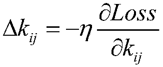
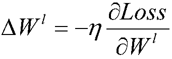
Blower fan blade fault identification method based on deep level characteristic extraction

Abstract

The invention discloses a blower fan blade fault identification method based on deep level characteristic extraction. The method comprises steps that an ImageNet image training depth learning neural network is collected to acquire a convolution kernel, a weight and a bias value, the size of a blower fan blade is further adjusted to the size same as an ImageNet image database, a prediction set and a training set are acquired through division, the training set is inputted into the depth learning neural network, and 4096 values of a previous layer of an output layer are extracted and are taken as characteristic values. All the 4096 characteristic values of the training sample are inputted to a support vector machine model for training, 4096 characteristic values of test machine blower fan blade images are further extracted through the depth learning model and are inputted to the trained support vector machine model, and the fault result is acquired. Blower fan blade fault types can be relatively well identified through pictures, management personnel is facilitated to make corresponding processing, and a management level of a wind power plant can be effectively improved.

Description

Fan Blade Fault Identification Method Based on Deep Hierarchical Feature Extraction technical field The invention relates to the technical field of fan blade image fault identification, in particular to a fan blade image abnormality recognition method based on depth-level feature extraction, and the fault type is judged through the fan blade picture. Background technique Modern social life is inseparable from energy. However, with the reduction of non-renewable energy such as petroleum, people are becoming more and more aware of the energy crisis and have begun to vigorously develop renewable energy. As one of the renewable energy sources, wind energy is widely distributed and has huge energy, so it has great application prospects. Fan blades are power components that convert wind energy into electrical energy, which directly affects the conversion efficiency of wind power generation. However, the blades are in the natural environment for a long time, and typhoons, rainsto...

AI Technical Summary

Problems solved by technology

With the continuous expansion of wind power generation scale, the traditional manual inspection can no longer meet the daily inspection needs of wind power generation, and the demand for efficient diagnosis methods for fan blade faults is becoming more and more urgent.

The traditional fault diagnosis method for wind turbine blades is manual inspection, which requires inspectors to climb up the wind turbine and rely on experience to judge the damage of the blades. However, for large-scale wind power stations, manual inspection is undoubtedly too inefficient

Recently, it is more popular to predict the power generation of wind turbines in combination with environmental factors, and compare the actual power generation of wind turbines to judge the damage degree of blades, but it cannot detect potential faults of wind turbine blades, and cannot predict failures before failures occur, nor can it judge Blade failure type

Images