[0056] Embodiment two
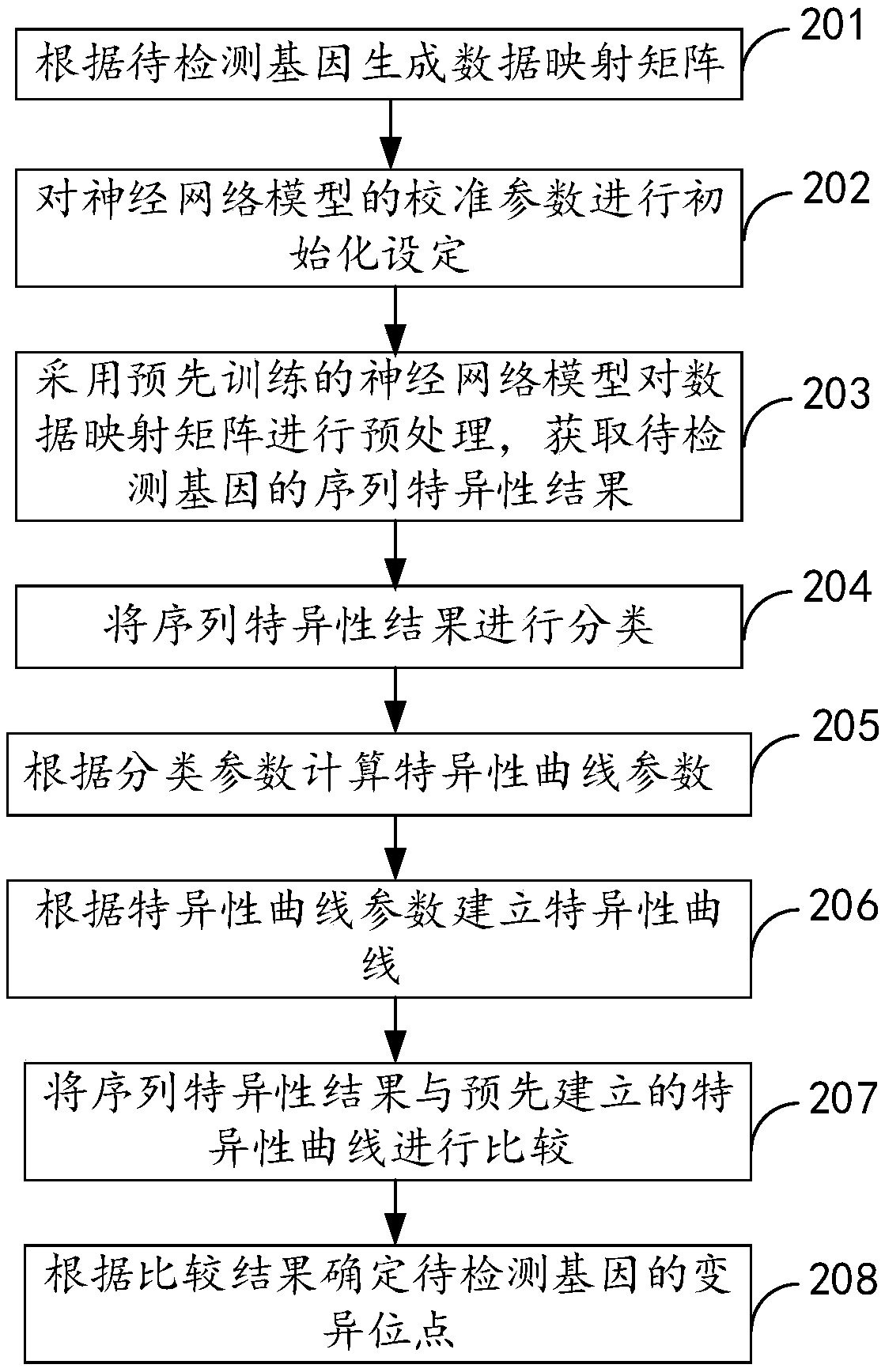
[0057] figure 2 It is the method for detecting gene mutation sites provided in Example 2 of the present invention. like figure 2 As shown, this embodiment provides a method for detecting gene mutation sites, including:
[0058] Step 201, generating a data mapping matrix according to the gene to be detected, specifically including:
[0059] 1) Extract the base sequence in the gene to be detected;
[0060] 2) determine the type of base sequence;
[0061] 3) Construct a data mapping matrix corresponding to the base sequence type.
[0062] It should be noted that DNA is a long molecule composed of two complementary four types of bases (ie A, T, G, C). DNA, that is, deoxyribonucleic acid, is a sugar (organic A common type of chemical compound), a phosphate group (containing the element phosphorus), and one of four nitrogenous bases (A, T, G, C). The chemical bonds linking nucleotides in DNA are always the same, so the backbone of the DNA molecule is very regular. It is the differences in A, T, C, and G bases that endow each DNA molecule with a different "personality."
[0063] Since the DNA base sequence only contains A, T, G, and C, a simple binary mapping is performed on A, T, G, and C to form a sequence matrix, in which different columns correspond to different types of bases. When the corresponding base appears, it is 1, otherwise it is 0, and finally a simple matrix containing only 0 and 1 is obtained, that is, the data mapping of the DNA sequence is completed. For example, if the DNA sequence we input is S={GACTAG}, it can be mapped into a 6*4 binary matrix as follows:
[0064]
[0065] From left to right, the bases corresponding to the four columns of the matrix are A, T, G, and C respectively.
[0066] To summarize the above mapping, it can be summarized as:
[0067] Assuming that the maximum length of the convolution kernel is m, you need to construct a matrix S of order (n+2m-2)*4, S satisfies:
[0068]
[0069] That is, when a certain base in the sequence belongs to a certain category of A, T, G, and C, the element at the corresponding position in the matrix is 1, otherwise it is 0, and when the base is uncertain, the complement is 0.25.
[0070] It should be noted that a more detailed division can also be performed, and no more examples are given here.
[0071] Step 202, initialize and set the calibration parameters of the neural network model.
[0072] Among them, the calibration parameters include the size of the convolution kernel, the number of convolution kernels, the initialization weight, the learning rate, the learning potential, and the processing scale.
[0073] Among them, the size and number of convolution kernels specifically include:
[0074] The size of the convolution kernel is determined by the length of the specific pattern of the DNA sequence.
[0075] Assume that we think that the specific pattern length of a base sequence is 4, and the types of base patterns are also 4, so the convolution kernel size should be 4*4=16. Combined with our past practical experience, we can know that it is more appropriate to choose a size that is 1.5 times larger than this.
[0076] We generally set the number of convolution kernels to 16, so that the best training effect can be obtained.
[0077] The parameter setting of the convolution layer should be as small as possible. First, it can increase the network capacity and the complexity of the model. Second, it can minimize the number of convolution parameters, and then cooperate with padding to make full use of the edge information of the input data.
[0078] The initialization weight and processing scale specifically include:
[0079] The neural network model generally relies on stochastic gradient descent for training and parameter update. The network performance is related to the optimal solution of convergence, and the convergence effect depends on the parameter initialization. The common initialization methods are as follows: all zero initialization, random initialization and so on.
[0080] The idea of all-zero initialization comes from the purpose of our model training, that is, when the model converges, the weights under ideal conditions basically maintain the same positive and negative states, that is, the expected value is 0, so all-zero initialization directly and roughly initializes the parameters Set all to zero. Then, in the case of all-zero initialization, since the outputs of different convolution kernels are exactly the same, the gradient update will also be completely converged, and the next round of update parameters will remain in the same state, and no changes can be made, that is, the training fails.
[0081] Random initialization is to set the parameter to a small random number close to 0, and the positive and negative are roughly half. Our models generally take a random initialization that follows a standard normal distribution.
[0082] The choice of processing scale determines the number of training samples involved in the calculation of the convolutional neural network each time the parameters are updated. Our model adopts a processing scale of 64 (batch_size=64).
[0083] The learning rate and learning potential specifically include:
[0084] Learning rate (learning rate) is an important parameter in model training. If it is selected properly, it can speed up the convergence of the model and improve the convergence efficiency. However, if it is not selected properly, there is a risk of "explosion" of the loss value of the objective function, resulting in training failure. . Based on mathematical derivation and estimation, the learning rate suitable for our model should be in the range of [0.0005, 0.5], generally 0.001 or 0.1.
[0085] Learning momentum is a fast gradient method based on learning rate. When a parameter changes towards the same trend at a steady rate during training, then we think it will continue to change towards this trend at this rate, so we can scale up its learning stride . Learning potential and learning rate have similar problems in the selection of size, so choosing an appropriate learning potential can also help speed up model training. We adopt the Nesterov type momentum random descent method, and the value range of the coefficient is between [0.95, 0.99].
[0086] Step 203, using the pre-trained neural network model to preprocess the data mapping matrix to obtain the sequence-specific results of the genes to be detected;
[0087] Among them, the pre-trained neural network model includes: convolutional layer, pooling layer, fully connected layer, Softmax function layer, one-hot encoding layer, and backpropagation layer.
[0088] Let the input DNA sequence be S, S={S 1 ,...S n}, the output is a numerical value, namely score(S), which is a compound function about S, score(S)=neural_network(pool(filter(conv(s)))).
[0089] Among them, the convolutional layer is specifically set as:
[0090] Given an input matrix S, a corresponding number of feature maps can be obtained after convolution operations with several motif detectors (ie, convolution kernels).
[0091] Assuming that the number of convolution kernels is d, the size of the output matrix X of this layer is (n+m-1)*d, and the matrix composed of all convolution kernels of this layer is M, and the order of M is d* m*4, then it can be obtained by weighted summation:
[0092]
[0093] Among them, M k,j,l Indicates the parameters of the kth convolution kernel at j.
[0094] The pooling layer is specifically set as:
[0095] The purpose of filtering is to sort the data of each column of the matrix in order from large to small, so as to retain the larger half of the elements, and use the activation function ReLU to linearly correct it to obtain the intermediate expression Y about X function.
[0096] Y is a matrix of the same order as X. After the maximum pooling, the dimension is reduced into a vector Z.
[0097] Z k =max{Y 1,K ,LY n,k},
[0098] where k∈{1,2,…,d}
[0099] The full connection layer is specifically set as:
[0100] The fully connected layer can convert the compressed vector Z output by the previous layer into a scalar score. If the dimension of the vector Z is d, and it is known that our fully connected layer contains 32 neurons, that is, d=32, then The score function that can be output is:
[0101]
[0102] The Softmax function layer is specifically set as:
[0103] The Softmax function is a function that converts each element in the training score array of the previous layer into the ratio of its exponent to the sum of the exponents of all elements, so as to greatly simplify subsequent operations. Because indexing is equivalent to enhancing the size characteristics of an element, even if the original large value is larger, it makes the original small value smaller, so it can approach the endpoints 0 and 1 faster. Therefore, we use softmax to map the obtained score to a probability value so that it falls between the interval [0.0, 1.0), the expression is:
[0104]
[0105] The specific setting of the one-hot encoding layer is:
[0106] For features with a specific number of values, after one-hot encoding, the output feature will also be converted into a specific number of binary features, with only one activation at a time. For example, if the number of DNA sequence feature types we know is m, then each output is a one-dimensional vector of length m, and the value of the element at the corresponding position is 1, and the value of the element at other positions is 0.
[0107] The backpropagation layer is specifically set as:
[0108] The output value after forward propagation is compared with the target value. After the prediction error is obtained, the error is reversely passed to the previous parameters to update the parameters until the parameters are close to the training set target and convergence is achieved.
[0109] For softmax mapping, the classification objective function we usually adopt is the cross entropy loss function, expressed as:
[0110]
[0111] Among them, L i is the target value of the known category.
[0112] By updating the error layer iteratively forward, you can get such a propagation path:
[0113]
[0114]
[0115] In this way, a backward propagation operation is completed by relying on the gradient descent method.
[0116] Among them, the pre-training uses the RNAcompete dataset.
[0117] According to research, the human genome and the genomes of many other eukaryotes encode hundreds of RNA-binding domains (RBD for short) containing classical sequence specificity and many other unconventional RNA binding proteins (unconventional RNA binding proteins, short for short). ucRBP) RNA-binding proteins (RNA-bindingproteins, referred to as RBPs).
[0118] RNAcompete's laboratory and data processing methods, a method previously used to analyze the RNA binding preferences of hundreds of RBD-containing RBPs from different eukaryotes, also determined the RNA binding of two human ucRBPs (NUDT21 and CNBP) preference.
[0119] In order to achieve a better training effect, the training data set uses the RNAcompete data set. The above data set consists of three parts: 1. Contains 213130 unique 29 to 38nt RNA sequence file sequences.tsv; 2. Contains the motif score file targets.tsv corresponding to each sequence; 3. The RNAcompete method found Motif collection file motif.
[0120] Optionally, after obtaining the sequence-specific results of the gene to be detected, it also includes:
[0121] Step 204, classifying the sequence-specific results;
[0122] Wherein, the classification parameters include: true positive, false positive, true negative, false negative.
[0123] After the sequence specificity is extracted, the following classification methods need to be adopted to classify the prediction results:
[0124] True positive (TP for short), that is, the feature is correctly hit;
[0125] False positive (false positive, referred to as FP), that is, wrongly hit the feature;
[0126] True negative (true negative, TN for short), that is, the feature is correctly missed;
[0127] False negative (FN for short), that is, falsely missing a feature.
[0128] Step 205, calculating specificity curve parameters according to classification parameters;
[0129] According to the above four classification parameters, the true positive rate is defined as the sensitivity:
[0130]
[0131] The false positive rate or specificity is:
[0132]
[0133] The precision is:
[0134]
[0135] In the formula, P is the positive rate and N is the negative rate.
[0136] Step 206, establishing a specificity curve according to specificity curve parameters.
[0137] Using the above data, the ROC curve was drawn with 1-specificity (1-FPR) as the horizontal axis and sensitivity TPR as the Y-axis.
[0138] Step 207, comparing the sequence specificity result with a pre-established specificity curve;
[0139] The concept of AUC (area under the curve of ROC) value is introduced, as an evaluation index of predictive performance, it is used to describe the size of the area enclosed by the ROC curve and the abscissa. Generally, the AUC value is in the [0,1] interval, and the performance of the AUC range classifier is positively correlated.
[0140] In the model training stage, the experimental data of RNAcompete shows that there are 291 kinds of motif features, and in the test stage of motif prediction, there are 244 kinds of motif sequences output, and the recognition rate is
[0141] We obtained 6130 groups of data on the binding probability of RNA and specific proteins, and compared them with the real values (1 is normal, 0 is variation), and used SPSS to draw the ROC curve of the convolutional neural network classifier, and obtained as follows image 3 ROC curve shown.
[0142] It can be seen that the AUC value of the classification model based on the convolutional neural network is 0.795, and the classification accuracy is relatively good.
[0143] Step 208, determine the variation site of the gene to be detected according to the comparison result.
[0144] When the above model is used to detect the test set with known motif features, it can effectively detect whether the output features of the corresponding positions are consistent with the known features, and if not, it can be inferred that there is a mutation at the position, that is Variation site.