Gravity inversion method based on cubic b-spline function
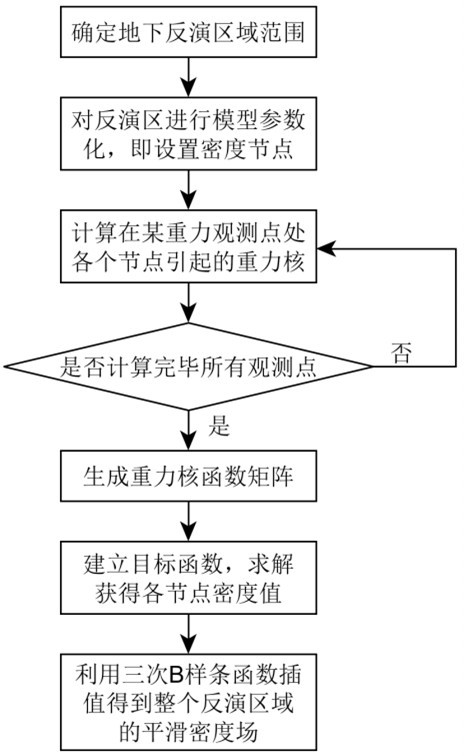
A spline function and gravity inversion technology, which is applied in the field of geophysical gravity exploration, can solve problems such as inability to invert smooth density field models, achieve reliable inversion results and avoid calculation errors
- Summary
- Abstract
- Description
- Claims
- Application Information
AI Technical Summary
Problems solved by technology
Method used
Image
Examples
Embodiment 1
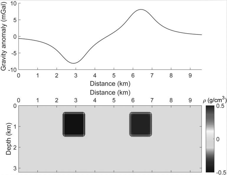
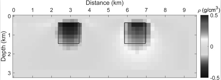
[0061] In order to illustrate the realization idea and implementation process of this method and prove the effectiveness of the method, the anomaly body (model 1) with density anomalies, one positive and one negative, is tested and compared with the results of conventional constant density unit L2 mode constrained inversion.
[0062] S1: will be as figure 2 Model 1 is shown as the true density model. The real density model is composed of a positive and a negative density anomaly, the two anomalous cross-sections are squares with a side length of 1.1 km, and the density difference is 0.5 g / cm 3 and -0.5g / cm 3 .
[0063] S2: Gravity observation points are arranged along the horizontal surface, with a distance of 100 m, and a total of 95 observation points.
[0064] S3: Calculate the gravity anomaly produced by model 1, such as figure 2 shown in the curve.
[0065] S4: The calculated gravity anomaly data is used as the observation data, the cubic B-spline node spacing is s...
Embodiment 2
[0071] In order to further illustrate the practicability of this method, three density anomaly bodies (model 2) of different sizes are tested, and compared with the results of conventional constant density unit L2 mode constrained inversion. Model 2 is composed of three positive density anomalies with different central buried depths and sizes. The cross-sections of the three anomalous bodies are squares with side lengths of 1.1 km, 0.6 km, and 0.3 km, respectively, and the density difference is 0.5 g / cm 3 ,Such as Figure 5 shown. Calculate the gravity anomaly produced by Model 2 as Figure 5 As shown in the curve, the inversion steps of Example 2 are the same as S4~S7 of Example 1. Image 6 is the inversion result of the conventional constant density element L2 mode constraint method. It can be clearly seen from the figure that the inversion density amplitude of this method is relatively small, the deeper the depth, the more divergent the density distribution, and the boun...
PUM
 Abstract
Description
Claims
Application Information