[0066] Example
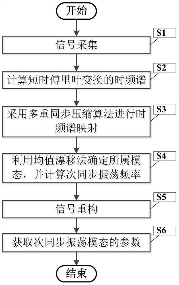
[0067] figure 1 It is a flowchart of a method for detecting subsynchronous oscillation of a high-proportion renewable energy power system according to the present invention.
[0068] In this example, if figure 1 As shown, the present invention is a method for detecting subsynchronous oscillation of a high-proportion renewable energy power system, comprising the following steps:
[0069] S1, signal acquisition;
[0070] Collect the voltage signal or current signal at the output end of the high-proportion renewable energy power system;
[0071] S2. Calculate the time spectrum of the short-time Fourier transform of the voltage signal or the current signal;
[0072] S2.1. Let the time-varying signal model of voltage signal or current signal be s(t):
[0073] s(t)=A(t)e iφ(t) (1)
[0074] Among them, A(t) represents the amplitude of the voltage signal or current signal, φ(t) represents the phase of the voltage signal or current signal, i is the imaginary number unit, and t is time;
[0075] S2.2. Carry out the first-order Taylor expansion of formula (1) to obtain:
[0076]
[0077] Among them, u is the integral variable, φ'(t) is expressed as the derivative of the phase with respect to time, and the local instantaneous frequency is obtained; then the signal s(t) can be expressed as:
[0078] s(t)=A(t)e i(φ(t)+φ'(t)(u-t)) (3)
[0079] Calculate the time spectrum G(t,ω) of the short-time Fourier transform of the signal s(t):
[0080]
[0081] Among them, g(·) is the window function, is the Fourier transform of the window function, ω is the frequency;
[0082] S3. Using a multiple synchronization compression algorithm to map the time spectrum of the short-time Fourier transform to a new time spectrum;
[0083] S3.1. Calculate the derivative of G(t, ω) with respect to time:
[0084]
[0085] S3.2. Calculate the instantaneous frequency of any point on the time scale domain
[0086]
[0087] S3.3. The time spectrum G(t,ω) obtained by short-time Fourier transform usually has serious energy divergence, which will cause unclear observation. Perform the first synchronous compression transformation on G(t,ω):
[0088]
[0089] Among them, δ( ) is the Dirichlet function, η is the frequency corresponding to a certain time t, Ts [1] (t, η) represents the synchronous compression transformation coefficient of s(t) on the time-frequency point (t, η) when the synchronization compression transformation is performed for the first time;
[0090] However, experiments have shown that the synchronous compression coefficient is not suitable for strong time-varying signal processing, so when subsynchronous oscillation occurs, the method of synchronous compression transformation of the time spectrum is continuously performed, and the equation of multiple synchronous compression transformation coefficients can be obtained, that is, the formula ( 7) The obtained time spectrum is subjected to synchronous compression transformation again, and after substitution, the coefficients after the second synchronous compression transformation can be obtained as follows:
[0091]
[0092] In the same way, the time-frequency spectrum obtained by formula (8) is used to perform synchronous compression transformation again, and so on, until m times of synchronous compression transformation are performed, and the coefficients after multiple synchronous compression transformations are obtained:
[0093]
[0094] S3.4, on the basis of the formula (9), calculate the estimated value of the instantaneous frequency after the multi-synchronous compression transformation;
[0095]
[0096] For each iteration, the MSTS will construct a new instantaneous frequency estimate to redistribute the energy of the fuzzy STFT. Obviously, through multiple iterations, the MSTS frequency estimate will get closer and closer to the signal's actual instantaneous frequency;
[0097] S3.5. Based on frequency merging, the signal can be mapped from the time scale domain to the time-frequency domain, so as to obtain the time-frequency information of the signal. Therefore, we arrange the coefficients after multiple synchronous compression transformations in sequence according to time t to form the mapped time-frequency domain. spectrum;
[0098] S4. Using the mean shift method to determine the mode to which the coefficients after the multi-synchronous compression transformation higher than the set threshold belong, and calculate the sub-synchronous oscillation frequency;
[0099] S4.1, set the threshold T o , in this example, the threshold T o set to 0;
[0100] According to the analysis results of the MSS process, it can be seen that the MSS coefficients from the same pattern are all concentrated around the same frequency, therefore, we can reduce the coefficients below the threshold T o All other MSCT coefficients of will be ignored and will be higher than the threshold T o The multi-synchronous compression transformed coefficients are mapped to X s (t,η):Ts [m] (t,η)→η, where X s (t, η) means belonging to the coefficient Ts [m] (t, η) is gathered in the set of all time-frequency points (t, η) of frequency η;
[0101] S4.2, use the mean shift method to X s (t,η) clustering to calculate the modal frequency of each class
[0102] Let X s The number of modes of (t,η) is N, χ n Indicates the nth category, n=1,2,...,N;
[0103] Calculate the modal frequencies of the nth class
[0104] The modal frequency can be calculated as the centroid of the corresponding aggregated multi-synchronous squashed transform coefficients, the specific calculation formula is:
[0105]
[0106] Among them, |·| means to find the absolute value;
[0107] S4.3. When the working frequency is 50Hz, it will meet the modal frequency with a frequency range of [5,45]Hz (when the working frequency is 60Hz, the subsynchronous oscillation frequency range is [5,55]Hz) Denoted as the subsynchronous oscillation frequency, the mode it belongs to is the subsynchronous oscillation mode;
[0108] S5. Signal reconstruction
[0109] Considering that the MSS only redistributes the time-frequency coefficients in the frequency direction and there is no information loss, the MSS can perfectly reconstruct the signal, so each mode can be reconstructed by the following formula:
[0110]
[0111] Wherein, b is the bandwidth of multiple synchronous compression transformation, and in the present embodiment, the bandwidth is 50Hz; g(0) is the value of the window function at 0, φ' n (t) represents the derivative of the phase of the nth mode to time;
[0112] Reconstructed signal of signal s(t) The superposition of signals is reconstructed for each mode, that is:
[0113]
[0114] S6. Estimating the reconstructed signal of the subsynchronous oscillation mode by the least squares estimation method to obtain the parameters of each subsynchronous oscillation mode;
[0115] S6.1. Define function G n (A n ,ε n ,θ n );
[0116]According to the idea of the least squares method, the best matching parameters are solved by minimizing the square sum of the difference between the modal reconstruction signal and the assumed parameters, that is, the modal parameters can be formulated as the following problem:
[0117]
[0118] in, is the oscillation frequency of each subsynchronous oscillation mode; A n is the corresponding amplitude, θ n is the phase angle and ε n is the damping coefficient; T s is the sampling interval of the current/voltage signal, in this embodiment, the sampling interval is set to 8.33 milliseconds, that is to say, the sampling frequency is 120 Hz; k=0, 1, 2, ... are different sampling points;
[0119] S6.2. Find the function G based on the least squares estimation algorithm n to A n ,ε n ,θ n Respectively, the parameter values when the partial differential is equal to 0, so as to obtain the subsynchronous oscillation mode parameters:
[0120]
[0121] Finally, the subsynchronous oscillation frequency, amplitude, damping coefficient and phase angle are obtained.
[0122] In order to facilitate those skilled in the art to understand the technical content of the invention, the content of the present invention will be further explained below in conjunction with the accompanying drawings. The present invention performs parameter identification of subsynchronous oscillation on an example signal of the IEEE second standard model (operating frequency is 60 Hz) as shown in Table 1.
[0123]
[0124] Table 1
[0125] Signal waveform such as figure 2 As shown in (a), similar to the collection of subsynchronous oscillation components, the subsynchronous oscillation is caused by the disturbance occurring at 0.5s and then cleared after 0.1s. Then, STFT, SST, and MSST are performed on the signal.
[0126] figure 2 (b), figure 2 (c) and figure 2 (d) is the result after processing by the three methods of STFT, SST and MSST, figure 2 (b) and figure 2 (c) is a plot according to SST coefficient and MSST coefficient. It can be seen that the instantaneous frequency components after the disturbance are concentrated on three frequencies. It can be clearly seen that the "pseudo" time-frequency representation composed of STFT and SST, such as figure 2 (b) and figure 2 As shown in (c), the blurred image is due to the "interference" from STFT and SST. The main frequency is 51Hz. To avoid interference from other frequencies, filters are used to decompose the signal into several subbands. Compared with other methods, there is no pseudo-time-frequency phenomenon in the signal after MSST processing, and the image is the clearest. Therefore, this method does not require those preprocessing measures.
[0127] processed according to MSST figure 2 The analysis results in (d), the number of modes can be easily determined by visual observation. However, for more effective recognition, we need an algorithm that can automatically obtain the number of patterns. from figure 2 (d) It can be seen that the MSST coefficients from the same mode are all concentrated around the same frequency. Therefore, we can define a mapping as features with MSST coefficients above a set threshold; all other MSST coefficients below this threshold are ignored. Then, cluster analysis was performed using these features to determine the number of modes to which the non-zero MSST coefficients belong and the frequency corresponding to the modes.
[0128] like figure 2 As shown in (d), considering that all clusters can be clearly distinguished, a linear kernel function is used when applying the mean-shift algorithm, which can also reduce the computational complexity. The modal numbers are determined by the mean-shift method, and the modal frequencies can be calculated as the centroids of the corresponding MSST coefficient clusters. To assess the detection frequency The accuracy of the result, we use the estimated error EE, given by:
[0129]
[0130] Among them, f n is the actual frequency;
[0131] For each detected mode, calculate the frequency and EE and recorded in Table 2. It can be seen from Table 2 that the modal frequency estimation is accurate, and the estimation errors of the three modes are all less than 1%.
[0132]
[0133] Table 2
[0134] Each modal signal is reconstructed. In order to evaluate the accuracy of the reconstructed signal, the signal-to-noise ratio (SNR) is introduced and calculated as follows:
[0135]
[0136] Among them, s n For each modality's raw signal, The reconstructed signal for each mode, found for Equation (12), is the reconstructed signal for each detected subsynchronous oscillation mode in the example, and is given in Table 3. In order to verify the anti-noise ability of the method, 20dB Gaussian white noise is added to the signal. The reconstruction accuracy is shown in the third row of Table III, indicating that the method can accurately reconstruct the individual components of the signal.
[0137]
[0138] table 3
[0139] The least squares method is used to identify the parameters of the reconstructed subsynchronous oscillation mode, and the results are shown in Table 4;
[0140]
[0141] Table 4