Multilevel analysis of self-similar network traffic
- Summary
- Abstract
- Description
- Claims
- Application Information
AI Technical Summary
Benefits of technology
Problems solved by technology
Method used
Image
Examples
example 1
[0068]This relates to a 3 level, 6 state MMPP model to simulate heavy traffic that is bursty and self-similar as shown in FIG. 6. The packet bursts are shown by the vertical arrow clusters 602, and the first time level is shown as 604, the second time level as 606, and the third time level as 608.
[0069]1. Use algorithm τA to analyze input stream and generate trace τ1={(Λ11, P11), (Λ12,P12), . . . ,(Λ1i,P1i)}.
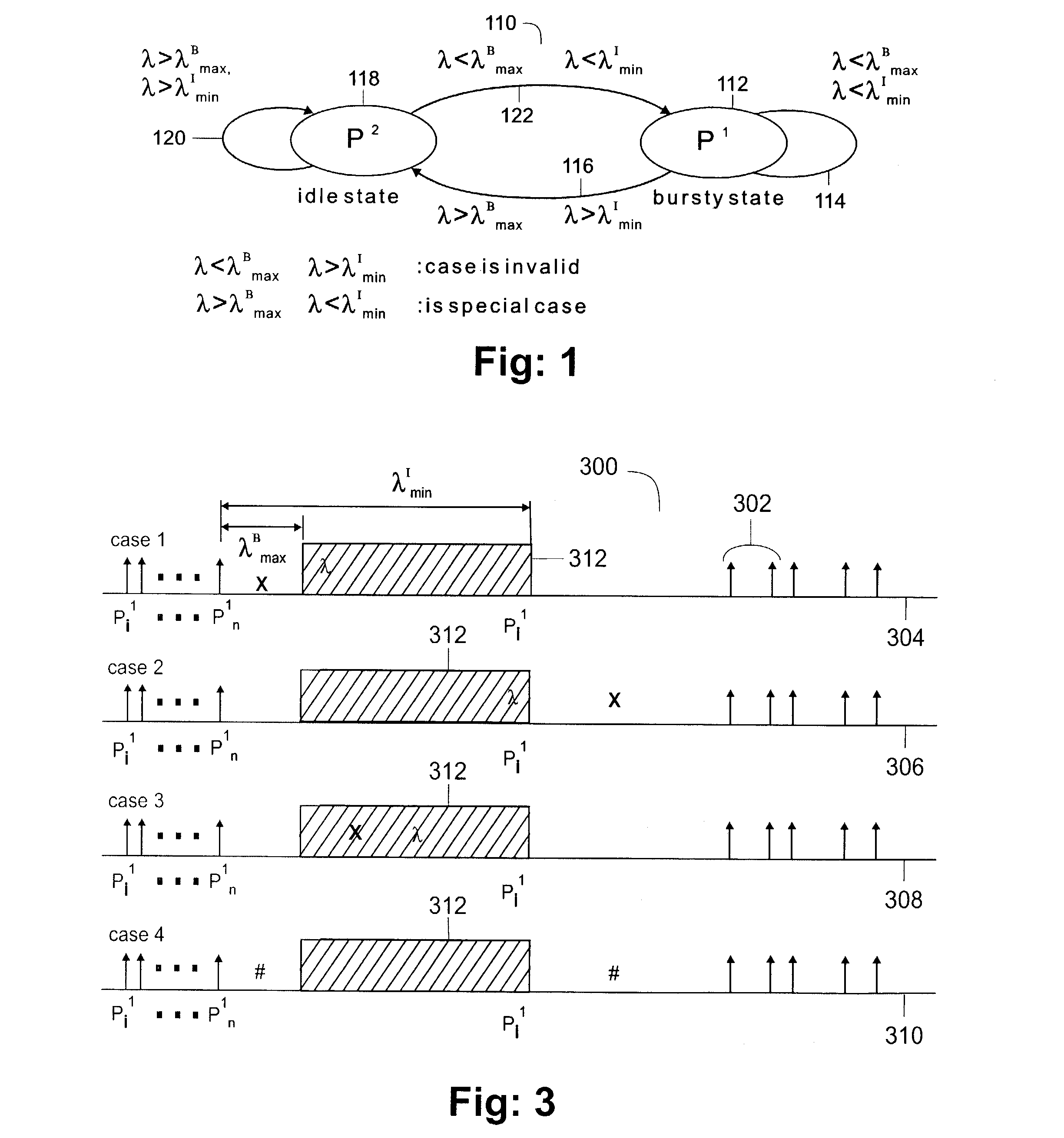
[0070]2. Analyze parameters Λ1i (the time stamp of leading of the packet), and P1i (the packet size) from trace τ1. From this the inter-arrival time λi is computed. Thus, there are four possible cases:
[0071]Case 1. λi1Bmax and λi1Imin: Pi is detected to belong to burst state PB.
[0072]Case 2. λi>λ1Bmax and λi>λ1Imin: Pi is detected to belong to idle state PI.
[0073]Case 3. λi>λ1Bmax and λi1Imin: Pi is detected to be inside of the transition window [λ1Bmax, λ1Imin]. In this case, the next state transition selected is dependent on the user process requirements.
[0074]Case 4. λi1Bmax ...
example 2
[0088]This relates to a 2-level, 4-state MMPP model to simulate heavy traffic that is bursty and self-similar, as shown in FIG. 7. The packet bursts are shown by the vertical arrow clusters 702. The first level is shown as 704 and the second level as 706.
[0089]Use algorithm τA to analyze input stream and generate trace τ1={(Λ11,P11),(Λ12,P12), . . . ,(Λ1i,P1i)}.
[0090]Analyze parameters Λ1i (the time stamp of leading of the packet), and P1i (the packet size) from trace τ1. From this the inter-arrival time is λi computed. As explained before, there are four cases are possible:
[0091]Case 1. λi1Bmax and λi1Imin: Pi is detected to belong to burst state PB.
[0092]Case 2. λi>λ1Bmax and λi>λ1Imin: Pi is detected to belong to idle state PI.
[0093]Case 3, 4: These cases are the same as for Example 1.
[0094]These four cases are used as the test criteria in algorithm s to generate Λ2i (the time stamp of leading of the burst), and P2i (the burst size). This analysis of trace τ1 generates trace τ2={...
example 3
[0100]This is directed to a 1-level, 2-state MMPP model to simulate heavy traffic that is bursty and self-similar, and is shown in FIG. 8. The packet bursts are shown by the vertical arrow clusters 802, and the only time level is shown as 804.
[0101]First, use algorithm τA to analyze input stream and generate trace τ1={(Λ11,P11), (Λ12,P12), . . . ,(Λ1i,P1i)}.
[0102]Then, analyze parameters Λ1i (the time stamp of leading of the packet), and P1i (the packet size) from trace τ1. From this the inter-arrival time is λi computed. As explained before, there are four cases are possible:
[0103]Case 1. λi1Bmax and λi1Imin: Pi is detected to belong to burst state PB.
[0104]Case 2. λi>λ1Bmax and λi>λ1Imin: Pi is detected to belong to idle state PI.
[0105]Case 3, 4: These cases are the same as for Example 1.
[0106]These four cases are used as the test criteria in algorithm τB to generate Λ2i (the time stamp of leading of the burst), and P2i (the burst size). This analysis of trace τ1 generates trace τ...
PUM
 Abstract
Description
Claims
Application Information


