Finite time convergence time-varying sliding mode attitude control method
An attitude control, limited time technology, applied in attitude control and other directions, can solve problems such as jumping and poor robustness, and achieve the effect of eliminating jumping problems and enhancing robustness.
- Summary
- Abstract
- Description
- Claims
- Application Information
AI Technical Summary
Problems solved by technology
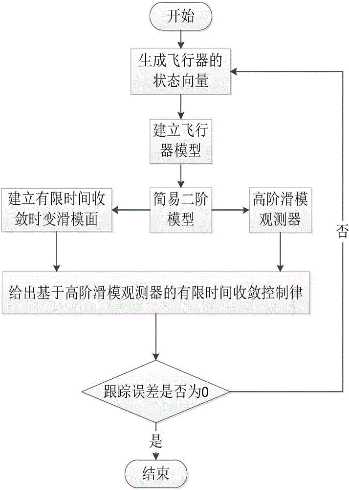
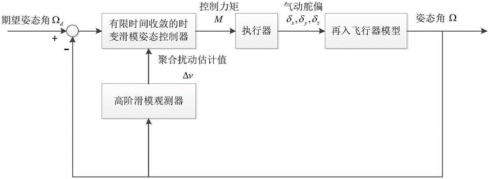
Method used
Image

Examples
Embodiment 1
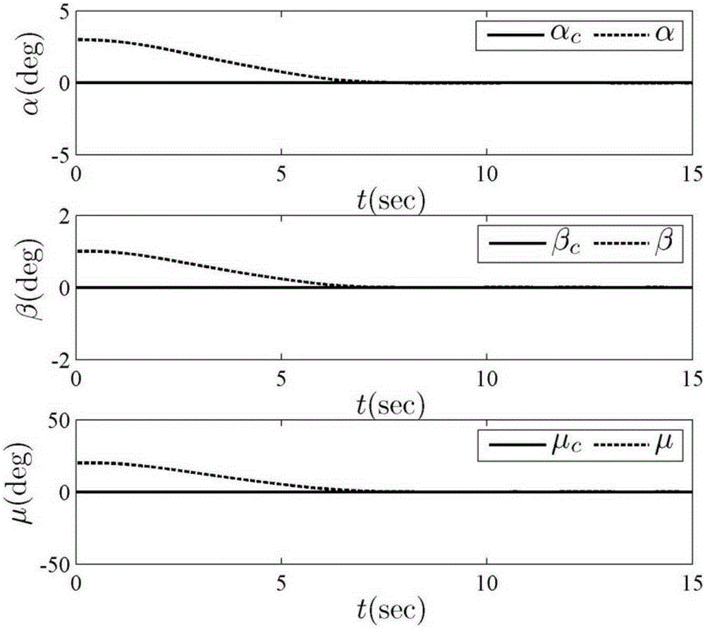
[0100] Using the hypersonic model of the Winged-Cone configuration announced by NASA as the simulation platform, the numerical simulation is carried out for its re-entry flight process. In the simulation, the initial altitude is 28km, the speed is 2800m / s, the initial attitude angle is [3120]deg, and the desired attitude angle is [000]deg. The initial attitude angular velocity is 0.
[0101] Since the flight conditions of the re-entry vehicle vary widely, and often have uncertainties such as aerodynamic parameter perturbation, for the problem of attitude control of the re-entry vehicle, it is necessary not only to test the control performance under nominal conditions, but also to test the control performance of the controller in In the case of drastic changes in environmental parameters and strong uncertainties in the system, whether robust and precise control can be performed. In order to further verify the robustness of the system, add a large external disturbance (directly...
PUM
 Abstract
Description
Claims
Application Information
PatSnap Eureka turns technology decisions into work you can execute. Powered by our Innovation Knowledge Graph, it runs expert workflows across engineering, life sciences, materials and intellectual property. Get your review-ready output in minutes.


