

Method for tracking and controlling locus of unmanned bicycle
A trajectory tracking and control method technology, which is applied in vehicle position/route/height control, non-electric variable control, position/direction control, etc., can solve the influence of bicycle trajectory, cannot obtain the best effect, cannot obtain tracking effect, etc. problem, the effect of achieving good results
- Summary
- Abstract
- Description
- Claims
- Application Information
AI Technical Summary
Problems solved by technology
Method used
Image

Examples
Embodiment Construction
[0069] A trajectory tracking control method for an unmanned bicycle proposed by the present invention will be described in detail below in conjunction with the accompanying drawings.
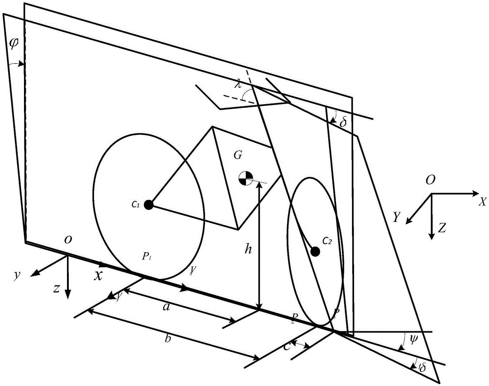
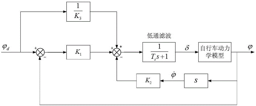
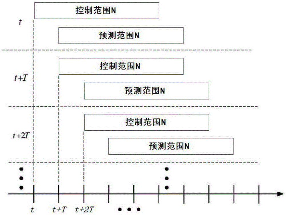
[0070] The invention implements the trajectory tracking control of the bicycle through a model predictive control algorithm. First, for the bicycle, establish its balance dynamics model, and establish the system state equation after adding the self-balancing controller; secondly, establish the kinematics model of the bicycle, and perform linearization; then combine the kinematics model with the self-balancing control system Combined with the corresponding simplified processing, a seven-dimensional state prediction model is established; finally, the linear quadratic index function is selected, its weight matrix parameters are set, and the optimal control input at each sampling time is solved online. Figure 8 It is a flow chart of the trajectory tracking control method of the unmanned bicycle of ...
PUM
 Abstract
Description
Claims
Application Information