Transformation apparatus, decision apparatus, quantum computation apparatus, and quantum machine learning system

Active Publication Date: 2019-06-27
NIPPON TELEGRAPH & TELEPHONE CORP
0 Cites 6 Cited by

AI-Extracted Technical Summary

Problems solved by technology

However, systems, such as deep neural networks, which have a wide industrial application range and in which development of their high-speed algorithms heavily affect society, are typically nonlinear.
Consequently, the systems cannot be efficiently learned using the HHL algorithm.
This is a problem similar to a lattice problem called LWE (learning ...

Method used

[0046]The present invention provides a novel quantum computation method that speeds up the learning in a feed-forward neural network. The learning of the weight of each layer in the feed-forward neural network can be reduced to a problem of solving a linear equation having errors. This is a problem similar to a lattice problem called LWE (learning with errors) used for next-generation post-quantum public-key cryptography and the like. Accordingly, first, a quantum computation apparatus that solves a lattice problem at high speed is described (a first embodiment to a fourteenth embodiment), and a learning system that applies the quantum computation apparatus to perform learning in the feed-forward neural network (fifteenth embodiment). The back propagation, which are typically used for learning in the feed-forward neural network, cannot get out from a local optimal solution in a learning process. Meanwhile, a learning system proposed in a fifteenth embodiment achieves improvement in speed by globally searching for an optimal solution through taking advantage of the characteristics of quantum physics. Note that the lattice problem dealt with in the present invention is an NP-hard problem. Consequently, the proposed method is applicable not only to learning in the feed-forward neural network but also widely to a wide variety of the combinatorial optimization problem.
[0081]The “dual lattice of modulo N” introduced in each embodiment is different from the general “dual lattice”. The dual lattice of modulo N is introduced because the result of execution of N-dimensional quantum Fourier transform to all coordinate axes in a state of superposition of lattices is a superposition of the dual lattice of modulo N. An LLL-reduced basis of the dual lattice of modulo N is called a “dual basis of modulo N”. Here, see pp. 33-35 of reference literature 1 for the definition of LLL-reduced basis. It has been known that application of LLL algorithm to any basis obtains a basis satisfying the definition of the LLL-reduced ...

Benefits of technology

[0012]As described above, the closest vector problem (CVP) about the basis B and the target vector t, and the learning with errors (LWE) of Formula (1) can be efficiently transformed into the pro...

Abstract

First, a dual basis B of B of modulo N is obtained by classical computation. Next, quantum computation is performed using the periodicity of a point sequence included in a sum set of sets obtained by parallel translation of a lattice L(B) by integral multiples of t for a plurality of integers, and an n-dimensional rj=(rj1, . . . , rjn) and rj0 are obtained for j=1 , . . . , m. Subsequently, by classical computation, the closest vector rj(c)=(rj1(c), . . . , rjn(c))∈L(B) of the n-dimensional vector rj, and the difference vector rj(d)=rj−rj(c)=(rj1(d), . . . , rjn(d)) corresponding to rj(c) are obtained.

Application Domain

Quantum computersMultiple digital computer combinations +3

Technology Topic

Parallel translationQuantum +4

Image

  • Transformation apparatus, decision apparatus, quantum computation apparatus, and quantum machine learning system
  • Transformation apparatus, decision apparatus, quantum computation apparatus, and quantum machine learning system
  • Transformation apparatus, decision apparatus, quantum computation apparatus, and quantum machine learning system

Examples

  • Experimental program(17)

Example

FIRST EMBODIMENT
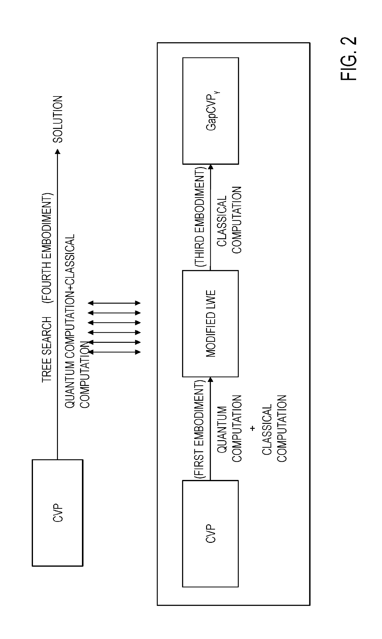
[0099]In a first embodiment, the CVP is transformed into the modified LWE by an operation (quantum computation) through a quantum computer and an operation (classical computation) through a classical computer (FIG. 2).
[0100]This embodiment has an object to transform the CVP into the modified LWE, which is a problem that can be computed at high speed on a quantum computer. Specifically, the parameters identifying the modified LWE problem corresponding to the input CVP are computed using the quantum computation and the classical computation.
[0101]A basic idea is described. In general, the lattice problem is believed to be difficult to be dealt with by the quantum computer, because the lattice problem has no periodicity with respect to the solution. However, the lattice has a structure symmetrical with respect to each lattice point. Accordingly, the periodicity with respect to the solution can be made. In this embodiment, quantum computation is performed using the periodicity of solution.
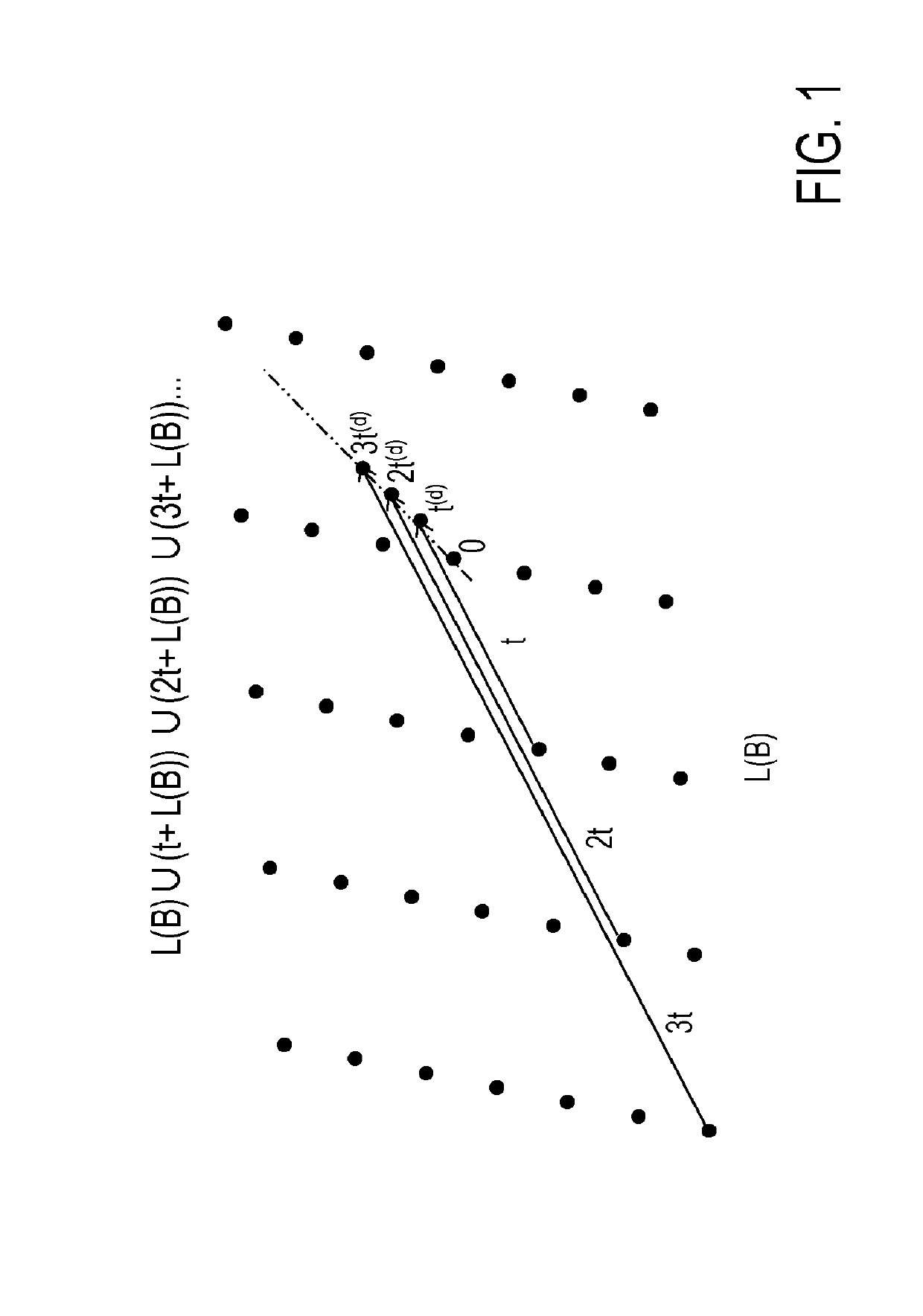
[0102]Specifically, the following method is adopted. The base is a method of solving the CVP. Let t(d) be the difference vector of solution of CVP for a pair (B, t). As exemplified in FIG. 1, the sum set L(B)∪(t+L(B))∪(2t+L(B))∪(3t+L(B))∪ . . . of L(B), t+L(B), 2t+L(B), 3t+L(B), . . . is a set where the point sequences are arranged at intervals of t(d). In consideration of viewability of the diagram, FIG. 1 exemplifies only the point sequence based on one lattice point. In actuality, the point sequences based on all the lattice points are arranged at intervals of t(d). In the quantum computation of this embodiment, information on the point sequence arranged at equal intervals is taken by executing quantum Fourier transform on the quantum computer. Subsequently, the CVP with respect to the taken information is solved by classical computation to obtain the modified LWE.
[0103]
[0104]As shown in FIG. 4, a transformation apparatus 1 of this embodiment includes classical computers 11 and 13 (first and second classical computers), a quantum computer 12, and a controller 14. The transformation apparatus 1 executes each process under control of the controller 14. The classical computers 11 and 13 include multiple arithmetic units (not shown). As exemplified in FIGS. 5 and 6, the quantum computer 12 includes an index register 121a, a data register 121b, a work register 121c, a quantum state generator 122, quantum Fourier transformation units 123a and 123b (first and second quantum Fourier transformation units), a manipulator 124, observers 125a to 125c, and an inverse quantum Fourier transformation unit 126. The transformation apparatus 1 includes processing circuitry configured to implement the classical computers 11 and 13 (first and second classical computers), the quantum computer 12, and the controller 14.
[0105]
[0106]The processes of this embodiment are described. The transformation apparatus 1 of this embodiment receives the basis B and the target vector t for CVP(B, t) as inputs, and outputs {rji(c),rji(d),rj0} and m, M and N, which satisfy the modified LWE of Formula (5).
( ( r 11 ( c ) … r 1 n ( c ) r 21 ( c ) … r 2 n ( c ) r 31 ( c ) … r 3 n ( c ) ⋮ ⋱ ⋮ r m 1 ( c ) … r mn ( c ) ) + ( r 11 ( d ) … r 1 n ( d ) r 21 ( d ) … r 2 n ( d ) r 31 ( d ) … r 3 n ( d ) ⋮ ⋱ ⋮ r m 1 ( d ) … r mn ( d ) ) ) ( t 1 ( d ) ⋮ t n ( d ) ) + ( e 1 e 2 e 3 ⋮ e m ) mod N = ( round ( r 10 N M ) round ( r 20 N M ) round ( r 30 N M ) ⋮ round ( r m 0 N M ) ) ( 5 )
The processes of this embodiment include classical computation (preprocess) by the classical computer 11, quantum computation by the quantum computer 12, and classical computation (postprocess) by the classical computer 13.
[0107]<
[0108]The classical computer 11 (FIG. 4) receives the pair (B, t) as an input, and executes the following processes.
[0109]1. The arithmetic unit of the classical computer 11 computes and outputs the least common multiple N′ of the denominators of the elements of the inverse matrix β−1 of the basis matrix β corresponding to the basis B (step S111).
[0110]2. The arithmetic unit of the classical computer 11 computes and outputs a dual basis B−′={b1−′, . . . , bn−′} of the basis B of modulo N′ (step S112).
[0111]3. The arithmetic unit of the classical computer 11 selects and outputs the multiple N of N′ (step S113).
[0112]4. The arithmetic unit of the classical computer 11 obtains and outputs the dual basis B−=(N/N′)B−′={(N/N′)b1−′, . . . , (N/N′)bn−′} of modulo N for the dual basis B−′ (step S114). The dual basis B− is “dual basis of modulo N” of the basis B.
[0113]5. The arithmetic unit of the classical computer 11 selects and outputs a positive integer M (step S115). M
[0114]6. The arithmetic unit of the classical computer 11 selects and outputs a real number R satisfying 2R≤N<4R (step S116).
[0115]7. The arithmetic unit of the classical computer 11 selects and outputs a positive real number L (step S117). L is an estimate of the length ∥t(d)∥ of the shortest difference vector t(d). For example, L×M
[0116]8. The arithmetic unit of the classical computer 11 selects and outputs a positive integer m (step S118).
[0117]9. The classical computer 11 outputs (L, n, M, N, R, B, t) (step S119).
[0118]That is, the classical computer 11 uses the classical computer to generate (L, n, M, N, R, B, t), which are parameters required to start computation on the quantum computer from the input (B, t).
[0119]<
[0120]The quantum computer 12 (FIGS. 4 to 6) receives (L, n, M, N, R, B, t) as inputs, sets (prepares) a register string that includes the index register 121a having ceil(log2 M) quantum bits, the data register 121b having n×ceil(log2 N) quantum bits, and the work register 121c having n×ceil(log2 det(β) quantum bits, and executes quantum computation m times on the string. The quantum computer 12 obtains the n-dimensional vector rj=(rj1, . . . , rjn)∈[0,N)n and rj0∈[0,M) at the j-th quantum computation, and outputs the vector. Note that i=1, . . . , n, j=1, . . . , m. The j-th quantum computation is hereinafter described. Here, m is a preset positive integer, and is required to have a larger value to increase the precision of the solution as the ratio between the closest vector and the second-closest vector becomes lower (the problem becomes more difficult). On the contrary, when the ratio between the closest vector and the second-closest vector is high, not so large value is required to be selected as m. For example, when the ratio between the closest vector and the second-closest vector is 4 or higher, m of 100 or larger can obtain a solution with a sufficiently high precision.
[0121]1. The quantum state generator 122 prepares a register string having the index register 121a, the data register 121b and the work register 121c in the following quantum states (step S122).
1 B R ∑ x ∈ B R 0 〉 x 〉 0 〉 ( 6 )
Note that BR represents a set of the point x∈Zn included in [0,N)n. For example, BR is a partial region of [0,N)n. BR is defined by the real number R, for example. Note that [0,N) is a half-open interval that is 0 or more and less than N. For example, BR represents a set of the point x∈Zn having a distance from a predetermined n-dimensional reference point NV/2=(N/2, . . . , N/2).
[0122]In other words, for example, BR represents a set of vector from the origin to the point x∈Zn. That is, BR={x∈Zn|∥x−Nv/2∥≤R}. FIG. 7A conceptually represents BR in a case of n=2. In the case of n=2, BR is a set of points belonging to a region encircled by a circle having a radius R centered on (N/2,N/2). Note that among three column vectors in Formula (6), the left |0 represents the quantum state of the index register 121a, the middle |x represents the quantum state of the data register 121b, and the right |0 represents the quantum state of the work register 121c.
[0123]2. The quantum Fourier transformation unit 123a executes M-dimensional quantum Fourier transform on the index register 121a (step S123a). Accordingly, the quantum state of the register string transitions (changes) to the following quantum state.
1 M B R ∑ w = 0 M - 1 ∑ x ∈ B R w 〉 x 〉 0 〉 ( 7 )
That is, the quantum state of the index register 121a changes to a superposed state of |w.
[0124]3. Given w∈ZM and x∈ZNn, (yw,x,1, . . . , yw,x,n) is defined as an n-dimensional vector having elements of rational numbers yw,x,1, . . . , yw,x,n that satisfy x−wt=yw,x,1b1+ . . . +yw,x,nbn. The manipulator 124 executes quantum manipulation that transforms the quantum state |w |x |0 into the quantum state in Formula (8), on the register string in the quantum state of Formula (7) obtained by the quantum Fourier transformation unit 123a (step S124).
|w |x |det(β)(yw,x,1−floor(yw,x,1)), . . . , det(β)(yw,x,n−floor(yw,x,n)) (8)
[0125]4. The observer 125c observes the work register 121c in the quantum state of Formula (8) obtained by the manipulator 124 (step S125c). The quantum states of the index register 121a and the data register 121b then change to
1 M ∑ w = 0 M - 1 ( 1 B R ⋂ ( L ( B ) + s + wt ( d ) ) ∑ x ∈ B R ⋂ ( L ( B ) + s + wt ( d ) ) w 〉 x 〉 ) ( 9 )
Note that s is an indefinite n-dimensional vector. Among the two column vectors in Formula (9), the left |w represents the quantum state of the index register 121a, and the right |x represents the quantum state of the data register 121b. The quantum state of the data register 121b represents the state obtained by parallel-translating the aforementioned sum set L(B)∪(t+L(B))∪(2t+L(B))∪(3t+L(B))∪ . . . in BR by the n-dimensional vector s (FIG. 1). While s is indefinite, the quantum state represents the sequence of points arranged in BR at intervals of t(d). It is desirable that the norm ∥s∥ of the n-dimensional vector s (e.g., the Euclidean norm ∥s∥ of s) be sufficiently small. Preferably, the product of ∥s∥ and M is less than ½ of the minimum value of the shortest vector in the lattice L(B). FIG. 7B conceptually shows the quantum state in a case of n=2.
[0126]5. The quantum Fourier transformation unit 123b executes n-dimensional quantum Fourier transform on the data register 121b in the quantum state of Formula (9) after observation by the observer 125c (step S123b).
[0127]As described above, the data register 121b includes n×ceil(log2 N) quantum bits. The n×ceil(log2 N) quantum bits are divided into in units of each ceil(log2 N) quantum bit. A subset of the data register 121b that includes in units of each ceil(log2 N) quantum bit is called a data sub-register 121b-i. The data register 121b has n data sub-register 121b-1, . . . , 121b-n. The quantum Fourier transformation unit 123b executes the N-dimensional quantum Fourier transform on the data register 121b in the quantum state of Formula (9) in units of each data sub-register 121b-i. Accordingly, the quantum state of the data register 121b is the superposed state of the vector sum t(c)+t(d) of the lattice point vector t(c) of the dual lattice L(B−)={Σi=1, . . . , n xib−i|xi∈Z,b−i∈B−} and the difference vector t(d). FIG. 7C conceptually shows the quantum state in a case of n=2.
[0128]6. The observer 125b observes the data register 121b in the quantum state obtained by the quantum Fourier transformation unit 123b, and obtains an observation result (rj1, . . . , rjn) (step S125b). rji is the observation result of the data sub-register 121b-i.
[0129]7. The inverse quantum Fourier transformation unit 126 executes M-dimensional inverse quantum Fourier transform on the index register 121a in the quantum state after observation by the observer 125b (step S126).
[0130]8. The observer 125a observes the index register 121a after the execution through the inverse quantum Fourier transformation unit 126, and obtains an observation result rj0 (step S126).
[0131]The quantum computation described above is executed for j=1, . . . , m, thereby obtaining rj=(rj1, . . . , rjn) and rj0 for j=1, . . . , m. The quantum computer 12 outputs rj and rj0, which are the observation results described above.
[0132]<
[0133]The classical computer 13 receives rj and dual basis B− of modulo N as inputs, obtains and outputs the closest vector rj(c)=(rj1(c), . . . , rjn(c))∈L(B−) of the n-dimensional vector rj and the difference vector rj(d)=rj−rj(c)=)rj1(d), . . . , rjn(d)), for the dual lattice L(B−)={Σi=1, . . . , n xiB−i|xi∈Z, b−i∈B−} and the n-dimensional vector rj=(rj1, . . . , rjn) (step S13).
[0134]Here, rj(c) and rj(d)are each an n-dimensional vector. That is, the classical computer 13 computes the solution of CVP(B−, rj) for the pair (B−, rj) of the dual basis B− of modulo N and the n-dimensional vector rj=(rj1, . . . , rjn). When the value of N is larger than the dimension number n (for example, when the value of N is exponentially larger than the dimension number n), an exact solution of CVP(B−, rj) of the n-dimensional vector rj obtained as described above can be obtained for the dual basis B− of modulo N using the classical computer (here, proof is omitted). For example, the classical computer 13 computes the closest vector rj(c) that is the exact solution of this CVP(B−,rj) and the difference vector rj(d) using the nearest plane algorithm, and outputs the computed result. It can be proved that when N is large with reference to n, ∥rj(d)∥ j(c) and the difference vector rj(d) can be obtained by the nearest plane algorithm.
[0135]It can be theoretically proved that the integers N, M and m, the observation result rj0, the closest vector rj(c)=(rj1(c)) , . . . , rjn(c)) and the difference vector rj(d)=(rj1(d), . . . , rjn(d)) obtained as described above satisfy Formula (5) for the difference vector t(d)=t−t(c)=(t1(d). . . , tn(d))T that is the solution of CVP(B, t), and a vector e=(e1, . . . , em)T having small integer elements corresponding to errors (here, proof is omitted). The transformation apparatus 1 outputs the integers N, M and m, the observation result rj0, the closest vector rj(c)=(rj1(c), . . . , rjn(c)) and the difference vector rj(d)=(rj1(d), . . . , rjn(d)), as information representing the modified LWE.

Example

SECOND EMBODIMENT
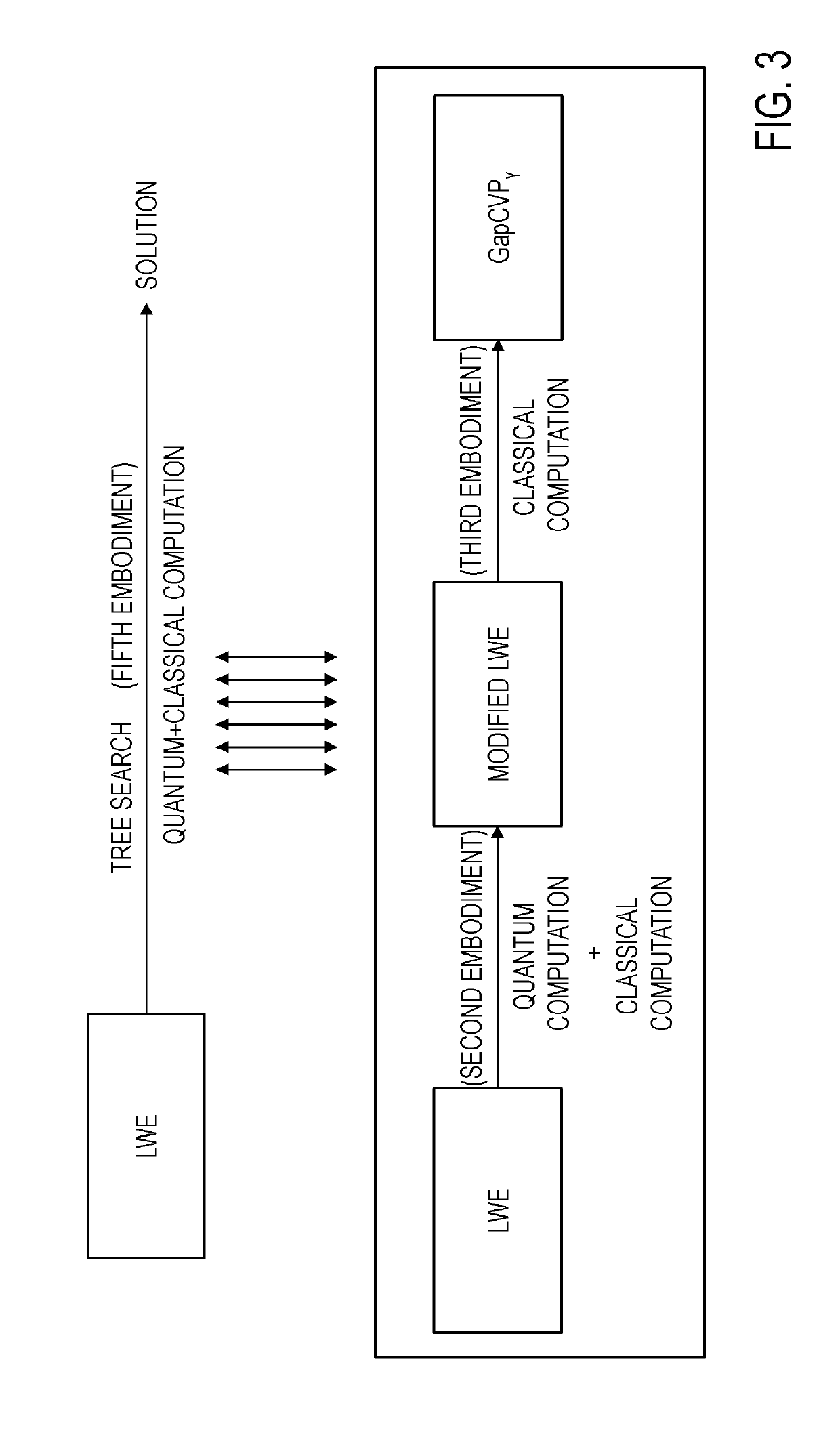
[0136]In a second embodiment, the LWE is transformed into the modified LWE by computation (quantum computation) through the quantum computer and computation (classical computation) through the classical computer (FIG. 3). Hereinafter, the difference from the first embodiment is mainly described. The same reference numerals are used for the items having already been described, and the description thereof is omitted.
[0137]As shown in FIG. 4, a transformation apparatus 2 of this embodiment includes classical computers 21 and 13 (first and second classical computers), a quantum computer 12, and a controller 14. The transformation apparatus 2 includes processing circuitry configured to implement the classical computers 21 and 13 (first and second classical computers), the quantum computer 12, and the controller 14.
[0138]The processes of this embodiment are described. The transformation apparatus 2 of this embodiment outputs {rji(c), rji(d),rj0} and m, M and N satisfying Formula (5) described above with t=g, for inputs that are the n-dimensional vectors aj=(a1j, . . . , anj)T and g=(g1, . . . , gn)T satisfying
( a 11 … a 1 m ′ a 21 … a 2 m ′ a 31 … a 3 m ′ ⋮ ⋱ ⋮ a n 1 … a nm ′ ) ( x 1 ⋮ x m ′ ) + ( d 1 d 2 d 3 ⋮ d n ) mod N ′ = ( g 1 g 2 g 3 ⋮ g n ) ( 10 )
representing LWE and the integer N′. The processes of this embodiment include classical computation (preprocess) by the classical computer 21, quantum computation by the quantum computer 12, and classical computation (postprocess) by the classical computer 13. The difference from the first embodiment is only the classical computation (preprocess) by the classical computer 21. Only the preprocess is hereinafter described.
[0139]<
[0140]The classical computer 21 (FIG. 4) receives (a1, . . . , am′, g, N′) identifying LWE, as inputs, and executes the following processes.
[0141]1. The arithmetic unit of the classical computer 21 sets an LLL-reduced basis computed from {a1, . . . , am′, N′ε1, . . . , N′εn} as the basis B, and outputs t=(t1, . . . , tn)T=g=(g1, . . . , gn) (step S211). Note that εu is an n-dimensional unit vector εu=(0, . . . , 1, 0, . . . , 0)T (u=1, . . . , n) that has the u-th element of 1 and the other elements of 0.
[0142]2. The arithmetic unit of the classical computer 21 computes and outputs a dual basis B−′={b1−′, . . . , bn−′} of the basis B of modulo N′ (step S112).
[0143]3.The arithmetic unit of the classical computer 21 selects and outputs a multiple N of N′ (step S113).
[0144]4. The arithmetic unit of the classical computer 21 obtains and outputs the dual basis B−=(N/N′)B−′={(N/N′)b1−′, . . . , (N/N′)bn−′} of modulo N for the dual basis B−′ (step S114).
[0145]5. The arithmetic unit of the classical computer 21 selects and outputs a positive integer M. M 115).
[0146]6. The arithmetic unit of the classical computer 21 selects and outputs a real number R satisfying 2R≤N<4R (step S116).
[0147]7. The arithmetic unit of the classical computer 21 selects and outputs a positive real number L. For example, L×M 117).
[0148]8. The arithmetic unit of the classical computer 21 selects (sets) and outputs a positive integer m (step S118).
[0149]9. The classical computer 21 outputs (L, n, M, N, R, B, t) (step S119).
[0150]Subsequently, the quantum computation by the quantum computer 12 and the classical computation (postprocess) by classical computer 13, which have been described in the first embodiment, are performed.

Example

THIRD EMBODIMENT
[0151]In a third embodiment, GapCVPγ for the modified LWE transformed in the first embodiment or the second embodiment is solved by the classical computation (FIGS. 2 and 3). That is, it is decided whether the difference vector t(d) satisfying Formula (5) identified by {rji(c), rji(d), rj0} and m, M and N obtained in the first embodiment or the second embodiment satisfies ∥t(d)∥≤L or satisfies ∥t(d)∥>γL.
[0152]
[0153]As exemplified in FIG. 8, a decision apparatus 3 of this embodiment includes a vector generator 31, a probability selector 32, a hyperplane distance estimator 33, a decision unit 34, and a controller 35. The decision apparatus 3 includes processing circuitry configured to implement the vector generator 31, the probability selector 32, the hyperplane distance estimator 33, the decision unit 34, and the controller 35. The decision apparatus 3 executes each process under control of the controller 35. As exemplified in FIG. 9, the hyperplane distance estimator 33 of this embodiment includes a basis generator 331, a vector generator 332, a hyperplane distance candidate setter 333, and a hyperplane distance selector 334.
[0154]
[0155]The processes of this embodiment are described. The decision apparatus 3 of this embodiment receives {rji(c), rji(d), rj0} and m, M and N as inputs, and outputs a decision result of decision of whether the difference vector t(d) satisfying Formula (5) identified by these inputs satisfies ∥t(d)∥≤L or satisfies ∥t(d)∥>γL. {rji(c), rji(d), rj0} and m, M and N are obtained by the processes described in the first embodiment or the second embodiment.
[0156]1. The vector generator 31 receives rj(c)=(rj1(c), . . . , rjn(c)) and rj(d)=(rj1(d), . . . , rjn(d)) as inputs, selects the n-dimensional vectors sj(c)=(sj1(c), . . . , sjn(c)) and sj(d)=(sj1(d), . . . , sjn(d)) that satisfy rj=rj(c)+rj(d)=sj(c)+sj(d) and sj(c)∈L(B−), and sets sj=sj(c)+sj(d) (step S31).
[0157]In this embodiment, sjn(d) is selected so as to satisfy ∥rj(d)∥≤∥sjn(d)∥≤2LN. It is defined as sj0=rj0.
[0158]2. The probability selector 32 selects and outputs the positive real number α and the probability q (step S32). In this embodiment, the probability selector 32 selects and outputs the probability q satisfying
0 q ≤ 2 π α Sin ( 2 π α ) + cos ( 2 π α ) - 1 π 2 α
[0159]The algorithm operates for any positive number α. A value recommended as α is a half-integer equal to or more than ½ and less than log n.
[0160]The hyperplane distance estimator 33 obtains an evaluation value Evalq based on the distance distj between the origin O and the hyperplane Hj that is the closest to the origin O among a finite number of hyperplanes whose normal vectors are the n-dimensional vectors sj(d) (the details of the process are described later) (step S33).
[0161]Here, it can be theoretically proved that any hyperplane Hj among the finite number (plurality) of hyperplanes whose normal vectors are the n-dimensional vector sj(d) corresponds to the difference vector t(d) (here, proof is omitted). A set of hyperplanes Hj whose normal vectors are sj(d) is obtained by parallel-translation of the vector space spanned by vectors that are elements of a subset of the lattice L(B), and includes a finite number of hyperplanes for each j. As exemplified as FIG. 10 (an example of n=2), such a set of a finite number of hyperplanes Hj are arranged at intervals of 1/∥sj(d))∥, and are arranged in a range of 2αN/M∥sj(d)∥ as a whole. Likewise, there are other hyperplanes that are arranged at intervals of 1/∥sj(d)∥ and arranged in the range of 2αN/M∥sj(d)∥ as a whole. These hyperplanes are repetitively arranged at intervals of N/∥sj(d)∥.
[0162]That is, as exemplified in FIGS. 11A and 11B (the example of n=2), the distal end of the difference vector t(d) is positioned on any of the hyperplane Hj of the finite number of hyperplanes whose normal vectors are the normal vector sj(d). As understood from these diagrams, the distance distj, between the hyperplane Hj closest to the origin and this origin, has correlation with the length (norm) of the difference vector t(d). Accordingly, even if the difference vector t(d) is unknown, the length of the difference vector t(d) can be evaluated on the basis of the distance distj. To perform this evaluation, the hyperplane distance estimator 33 obtains the evaluation value Evalq based on the distance distj for j=1, . . . , m.
[0163]The evaluation value Evalq in this embodiment is any of distances dist1, . . . , distm. In this embodiment, too large distances distj are excluded as errors, and the largest distance distj among the remaining distances distj is set as the evaluation value Evalq. The probability q described above serves as a reference to select the distance distj for excluding as errors. FIG. 12 exemplifies the relationship between the evaluation value Evalq and ∥t(d)∥/L. In FIG. 12, the ordinate axis represents the evaluation value Evalq, and the abscissa axis represents ∥t(d)∥/L. As understood from this diagram, evaluation of the magnitude of the evaluation value Evalq can decide whether to satisfy ∥t(d)∥≤L or satisfy ∥t(d)∥>γL.
[0164]4. The decision unit 34 receives the evaluation value Evalq as an input, outputs information that ∥t(d)∥≤L is satisfied when Evalq≤L is satisfied, and outputs information that ∥t(d)∥>γL is satisfied when EvalqL is satisfied (step S34).
[0165] 33
[0166]Details of processes of hyperplane distance estimator 33 are exemplified.
[0167]First, the hyperplane distance estimator 33 performs the computations of the following (a) to (c) for each j=1, . . . , m, and decides each distance distj.
[0168](a) The basis generator 331 (hyperplane basis generator) obtains the basis Bsj of the lattice {ν∈Zn|j, ν>=0 mod N} for the n-dimensional vector sj (step S331). The Hermite normal form is used for the computation of the basis Bsj.
[0169](b) The vector generator 332 obtains and outputs the n-dimensional vector bsj(d),N satisfying <
[0170](c) The hyperplane distance candidate setter 333 performs the processes of the following (i) to (iv) for y0=floor((sj0−α)N/M)+1 and y1=ceil((sj0+α)N/M)−1 (step S333).
[0171](i) The hyperplane distance candidate setter 333 obtains and outputs the n-dimensional vectors tsj,y0 and tsj,y1 that satisfy j, tsj,y0=y0mod N and j, tsj,y1=y1 mod N. The extended Euclidean algorithm is used for this computation.
[0172](ii) The hyperplane distance candidate setter 333 obtains and outputs the n-dimensional vectors t′sj,y0 and t′sj,y1 that satisfy t′sj,y0∈(sj+L(B))∩(tsj,y0+L(Bsj)) and t′sj,y1∈(sj+L(B))∩(tsj,y1+L(Bsj)). The Smith normal form is used for the computation.
[0173](iii) The hyperplane distance candidate setter 333 sets k minimizing ABS(j(d),t′sj,y0+kbsj(d),N) as ky0, sets k minimizing ABS(j(d),t′sj,y1+kbsj(d),N y1, and obtains and outputs t″sj,y0=t′sj,y0+ky0bsj(d),N and t″sj,y1=t′sj,y1+ky1bsj(d),N.
[0174](iv) The hyperplane distance candidate setter 333 outputs a hyperplane distance candidate distj=0 when j(d), t″sj,y0≤0≤j(d), t″sj,y1 or j(d), t″sj,y1≤0≤j(d), t″sj,y0 j(d), t″sj,y0 and j(d), t″sj,y1 are positive (j(d), t″sj,y0 and j(d), t″sj,y1 are larger than 0) or negative (j(d), t″sj,y0 and j(d), t″sj,y1 are smaller than 0), the hyperplane distance candidate setter 333 obtains and outputs ABS(j(d), t″sj,y0) or ABS(j(d), t″sj,y0), whichever is smaller, as the distance distj. That is, distance distj=min(ABS(sj(d), t″sj,y0), ABS(j(d), t″sj,y1)) is obtained and output.
[0175]The probability q set in step S32 and the distances dist1, . . . , distm obtained in steps S331 to S333 are input into the hyperplane distance selector 334. The hyperplane distance selector 334 obtains and outputs the floor(qm)-th value among the distances dist1, . . . , distm arranged in an ascending order with respect to the probability q, as the evaluation value Evalq∈{dist1, . . . , distm}. That is, the hyperplane distance selector 334 computes
Evalq=max({distj|j=1, . . . , m}, q)
(step S334).

PUM

no PUM

Description & Claims & Application Information

We can also present the details of the Description, Claims and Application information to help users get a comprehensive understanding of the technical details of the patent, such as background art, summary of invention, brief description of drawings, description of embodiments, and other original content. On the other hand, users can also determine the specific scope of protection of the technology through the list of claims; as well as understand the changes in the life cycle of the technology with the presentation of the patent timeline. Login to view more.

Similar technology patents

Micromirror element and optical switch

ActiveUS20050220394A1problem be solve
Owner:FUJITSU LTD

Display tilting apparatus

ActiveUS20050205735A1problem be solve
Owner:FUJITSU FRONTECH LTD

Image projection device

InactiveUS20110194035A1problem be solve
Owner:MITSUBISHI ELECTRIC CORP

Classification and recommendation of technical efficacy words

Why Eureka
Try Eureka