

3D model retrieval method and 3D model retrieval apparatus based on slow increment features
A slow-increment feature and 3D technology, applied in character and pattern recognition, special data processing applications, instruments, etc., can solve problems such as sudden changes in feature forms, achieve the effects of reducing difficulty, efficient and accurate retrieval results, and improving matching efficiency
- Summary
- Abstract
- Description
- Claims
- Application Information
AI Technical Summary
Problems solved by technology
Method used
Image

Examples
Embodiment 1
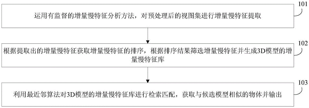
[0049] In order to make model retrieval more accurate, it can improve the efficiency of model retrieval and reduce the impact of external factors on the visual characteristics of the view. See figure 1 , this method includes the following steps:
[0050] 101: Using Supervised Incremental Slow Feature Analysis Methods [6] , perform incremental slow feature extraction on the preprocessed view set;
[0051] 102: Obtain the sorting of incremental slow features according to the extracted slow incremental features, filter the slow incremental features according to the sorting results, and generate a slow incremental feature library of the 3D model;
[0052]103: Use the nearest neighbor algorithm to retrieve and match the incremental slow feature library of the 3D model, and obtain and output objects similar to the candidate model.
[0053] Wherein, the method further includes: acquiring a 2D view set V of objects in the database, and preprocessing the 2D view set so that all 3D mo...
Embodiment 2
[0064] The scheme in embodiment 1 is described in detail below in conjunction with specific calculation formulas and examples, see below for details:
[0065] 201: Obtain the 2D view set V of the object in the database;
[0066] This method mainly uses the retrieval technology based on image comparison, that is, the 3D model is collected from multiple perspectives to form a 2D view set, and the mature 2D technology is used to extract the features of the object. Therefore, each 3D model is represented by multiple views, so the view set can be expressed as where v i Represents the view set of the i-th object; D represents the feature dimension of the view; f k Indicates the kth viewing angle of an object; N indicates the number of 3D models; M indicates the number of views of each 3D model; Indicates the scope to which each object's view collection belongs.
[0067] 202: Perform normalized preprocessing on the view set, so that the view sizes of all 3D models are consisten...
Embodiment 3
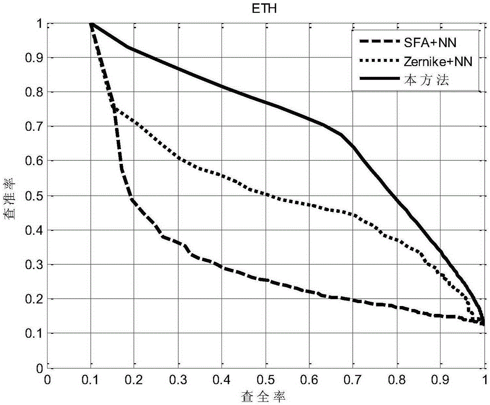
[0114] In this experiment, the embodiment of the present invention adopts the existing, online shared, more commonly used Zurich Federal Institute of Technology (German name The Technische Hochschule Zürich (ETH for short) database and the Taiwan University of China (NTU for short) database were used for experiments. The ETH database was relatively small and the models were more standardized, including 80 3D models, with a total of 8 categories and 10 objects in each category, namely apples and cars. , cow, mug, puppy, horse, pear, tomato. The NTU database has a total of 549 objects, 47 categories, and the number of objects in each category varies. The database is a virtual model database, and images are captured through 3D-MAX. This laboratory uses 60 virtual cameras to acquire images from different perspectives , each object obtains 60 views of different viewing angles, wherein the number of virtual cameras, that is, the shooting angle, can be set according to experimental ...
PUM
 Abstract
Description
Claims
Application Information