Dynamic capacity prediction method for overhead transmission line
A technology of overhead transmission line and prediction method, applied in the field of dynamic capacity prediction of transmission lines, can solve problems such as limited input, and achieve the effect of improving dimension and accuracy
- Summary
- Abstract
- Description
- Claims
- Application Information
AI Technical Summary
Problems solved by technology
Method used
Image

Examples
Embodiment Construction
[0041] The present invention will be further described below in conjunction with the accompanying drawings and embodiments.
[0042] A method for predicting the dynamic capacity of an overhead transmission line, comprising the following steps:
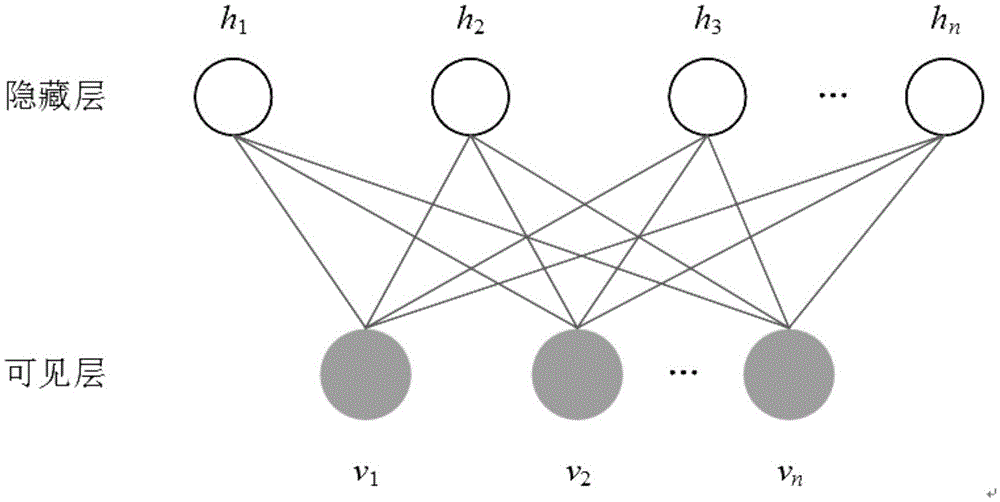
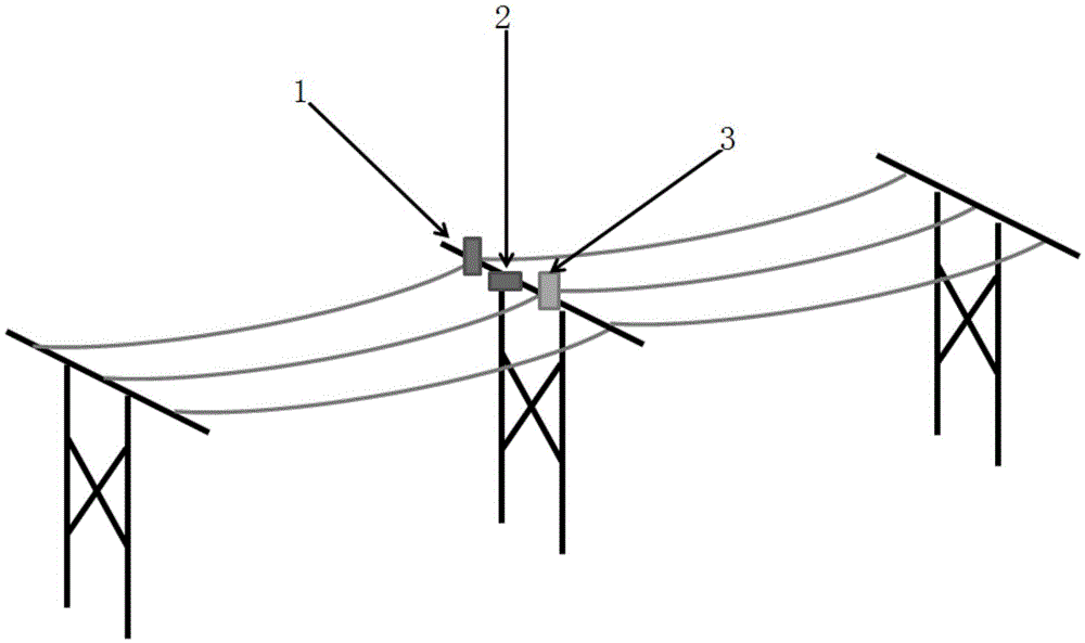
[0043] Step one, such as image 3As shown, the wind speed RMB deep learning machine is trained using the wind speed data collected by the wind speed sensor 3 on the iron tower and the meteorological forecast wind speed data provided by the National Meteorological Information Center, and the wind speed RMB is used to calculate the total energy of the wind speed RMB iteratively until the total energy of the wind speed RMB is for each learning sample When both reach the minimum value, the training of the wind speed RMB deep learning machine is completed;
[0044] Step 2, the wind speed at the current moment collected by the wind speed sensor 3 on the iron tower and the meteorological forecast wind speed are input into the wind speed RMB ...
PUM
 Abstract
Description
Claims
Application Information