Reference clock recovery for "eye" measurements

Active Publication Date: 2007-06-14
TEKTRONIX INC
11 Cites 10 Cited by

AI-Extracted Technical Summary

Problems solved by technology

In serial data communications an “eye” diagram is used to visualize how the signals used to transmit multiple bits of data representing a serial data stream may potentially lead to errors in the interpretation of the data bits.
This problem is known as inter-symbol interference.
The drawback of this method, as shown in FIG. 1, is that the resulting “eye” diagram using the recovered clock includes both high and low frequency jitter, with the low frequency jitter (wander) being reflect...

Abstract

A method for recovering a clock from a serial data stream for use in producing “eye” diagram measurements includes determining an initial recovered clock from the serial data stream based upon transition edges. Time interval error values are then determined as a function of the transition edges and corresponding initial recovered clock times. Time interval error values are interpolated for initial recovered clock times not associated with transition edges to produce a complete set of time interval error values. The complete set of time interval error values are lowpass filtered to produce a filtered set of time interval error values. The clock for the serial data stream is reconstructed from the filtered set of time interval error values.

Application Domain

Multiplex system selection arrangementsError prevention +8

Technology Topic

Clock recoveryReal-time computing +5

Image

  • Reference clock recovery for "eye" measurements
  • Reference clock recovery for "eye" measurements
  • Reference clock recovery for "eye" measurements

Examples

  • Experimental program(1)

Example

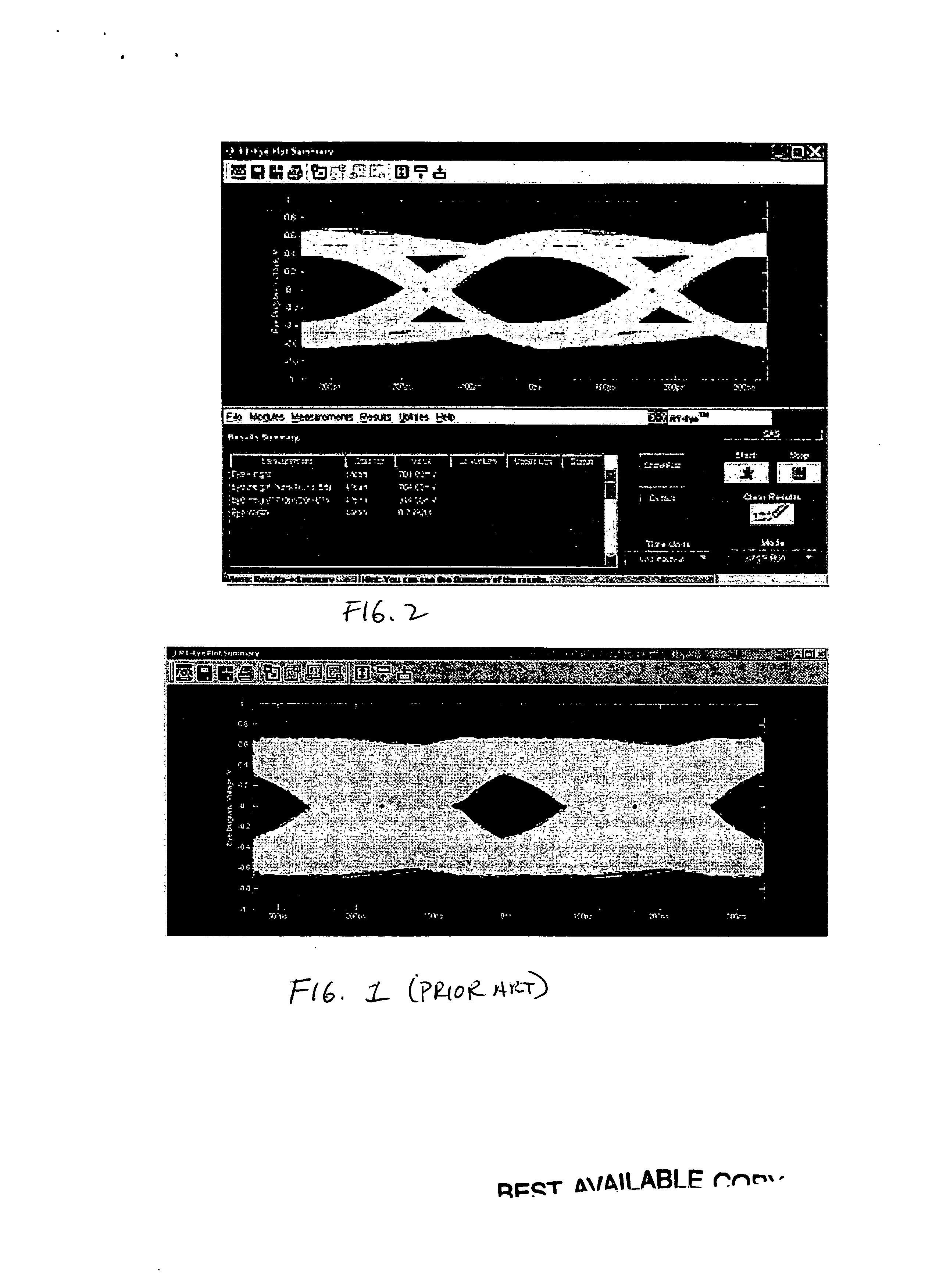
[0020] The “eye” diagram using only a constant clock recovery (CCR) method, shown in FIG. 1, has a lot of wander that is reflected as overall jitter on the “eye” diagram, as discussed above, whereas the “eye” diagram using a wander-tracked clock as recovered according to the present invention, shown in FIG. 2, reflects only the high frequency jitter.
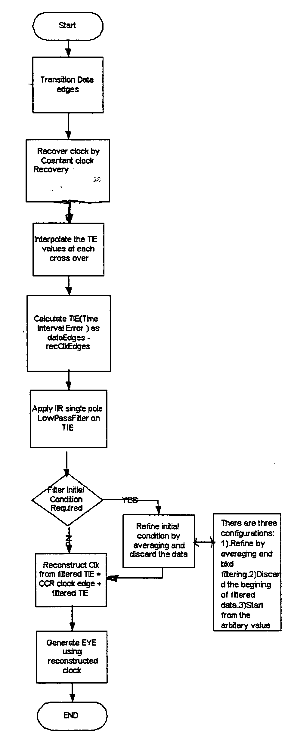
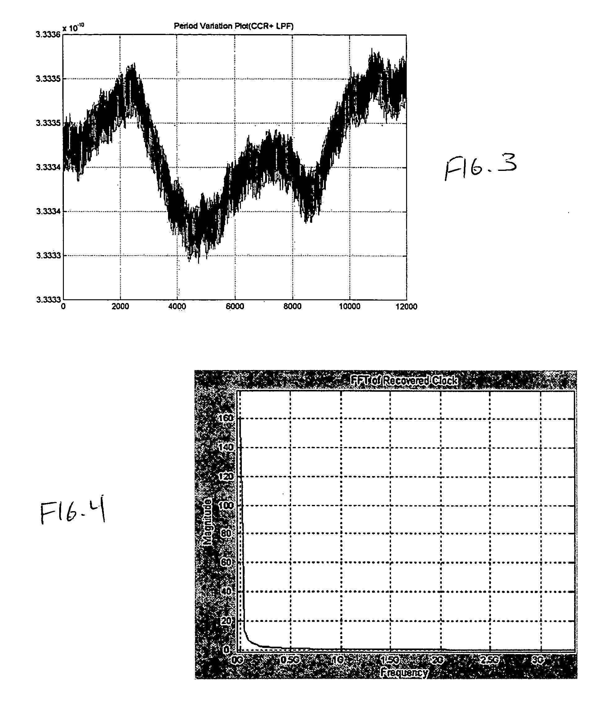
[0021] The CCR algorithm as described in U.S. Pat. No. 6,836,738 is used to calculate a recovered clock. CCR is done by using a least square fit algorithm applied to transition time intervals with a pre-defined data rate. The difference between the estimated clock transition times and the actual transition times is time interval error (TIE). The calculated TIE values have both high and low frequency jitter components, and are available at the actual data transitions. The transitions may not happen at the data rate, such as for non-return to zero (NRZ) data, and depend upon the bit encoding of the serial data stream. So intermediate TIE values at each estimated intermediate unit interval between signal transition times are calculated using a linear interpolation.
[0022] The complete set of TIE values are passed through an infinite impulse response (IIR) first order lowpass filter (LPF), such as a Butterworth filter designed with a cut-off frequency of fBAUD/1667 as specified in the T.10 Specification Guide, in order to remove the high frequency content. FBAUD depends on a device usage model and represents a signal speed of 1.5 Gbs and 3.0 Gbs. The purpose of using the LPF is to remove the high frequency jitter and retain all the low frequency jitter, i.e., wander, of the TIE values. The recovered clock by CCR is corrected by adding the low frequency jitter, which is equivalent to tracking the wander.
Reconstructed_Clock=CCR_Clock_Transitions+LPF(TIE)
The design details and calculation of filter coefficient variables that are used in the implementation of the single pole (first order) Butterworth LPF are referenced from standard text books as mentioned in Digital Signal Processing: A Practical Approach, 2nd Edition, by Emmanuel C. Ifeachor and Barrie W. Jervis published by Prentice Hall (2001), ISBN: 0201596199.
[0023]FIG. 3 shows a unit interval or clock period difference plot using the reconstructed clock which shows that the reconstructed clock is following the wander, while FIG. 4 shows a fast Fourier transform of the reconstructed clock with the high frequency jitter components above the cut-off frequency removed.
[0024] A graph of the filter response is shown in FIG. 5. Initially the filter ramps up and then tries to settle down after a few time constants indicated by the vertical dotted line. The first portion of the response is dominated by an initial condition response that typically takes a few time constants to settle. The time constant is determined by the smallest pole (eigenvalue) of the system, i.e., in the case of a first order filter by its cut-off frequency. The duration from the starting point to the vertical dotted line is called “transition time”, denoted as Td. The initial ramping up indicates how initial conditions are used for the filter behavior. During this initial ramping up there may be significant error between the input and output of the filter, and thus there is a need to overcome the transient effect of the filter. The simplest method is to discard the Td time duration of filter outputs.
[0025] There are different configurations to handle initial filter conditions to overcome the transient response of the filter. [0026] 1. Averaging and backward filtering technique: Calculate the initial state of the filter using the first 2.0 time constants of data and further refine the initial filter conditions using backward filtering. The 2.0 time constants are derived after experimenting with different waveforms and this value optimally calculates the initial conditions. Four point averaging is done on the first sample point until the 2.0 time constant of data. Using the last sample averaged value as the initial condition for backward filtering, do the backward filtering from the 2.0 time constant sample points to the first sample point. The filtered initial value is used as the initial condition for forward filtering. [0027] 2. Discarding the beginning of the filtered data: Configure the desired data points to be discarded after filtering as a time constant value. This configuration is provided as the transient time. The range of one time constant to ten time constants is provided depending on the signal speed 1.5 Gbs and 3 Gbs. [0028] 3. Both discarding and averaging: Select both of the above options to provide better filter initial condition handling. By selecting both the initial condition is calculated by averaging and backward filtering and then discarding the configured amount of data. Both options help to discard minimum data because initial conditions are already calculated. [0029] 4. Starting from an arbitrary value: If the above options are not selected, then the initial condition for filtering is from an arbitrary (first sample value) sample.
[0030]FIG. 6 shows an “eye” diagram spread due to the transient response of the filter which appears as more jitter by spreading the first few sample points. The resulting “eye” diagram may violate an applied mask. On the other hand FIG. 7 shows a clean “eye” diagram rendered by using the averaging technique for the initial filter conditions as described above.
[0031] In summary the clock recover algorithm is shown in FIG. 8. The transition data edges are detected and a recovered clock is determined using the CCR technique of U.S. Pat. No. 6,836,738. This provides time interval error values at each transition point of the input signal. In order to populate the subsequent filter, TIE values are interpolated for each clock point, i.e., edges are interpolated for each clock cycle not corresponding to an actual signal transition. The full set of TIE values are then lowpass filtered to eliminate the high frequency jitter component, and the clock is then reconstructed from the filtered TIE values. If TIE values are required for the part of the waveform where filter initial conditions dominate, then the initial condition is refined by one of the methods described above before reconstructing the clock from the filtered TIE values. The “eye” diagram for measurements is then generated using the reconstructed clock.
[0032] Thus the present invention provides a reconstructed clock from the serial data stream that tracks the signal wander so that a resulting “eye” diagram is produced that shows only the high frequency jitter for measurement.

PUM

no PUM

Description & Claims & Application Information

We can also present the details of the Description, Claims and Application information to help users get a comprehensive understanding of the technical details of the patent, such as background art, summary of invention, brief description of drawings, description of embodiments, and other original content. On the other hand, users can also determine the specific scope of protection of the technology through the list of claims; as well as understand the changes in the life cycle of the technology with the presentation of the patent timeline. Login to view more.
Why Eureka
Try Eureka