Adaptive range filters for range and point queries

Abstract

The technique described herein provides a way to summarize data and can also minimize unnecessary accesses to a data store. In one embodiment, the technique creates and stores an adaptive range filter that contains a compact summary of the contents of an index for a data store in the form of a trie data structure. Before accessing the index of the data store in response to a query, the technique checks the filter to determine whether the data store does not contain any keys for a specific range of data. If the adaptive range filter indicates that the index contains no keys satisfying the query predicate, the index of the data store and the data itself is not accessed. The adaptive range filter of the technique supports both range predicates and equality predicates. It is adaptive to changes in data and queries by learning the query and data distribution.

Description

BACKGROUND[0001]Data storage is becoming more and more important in a world that heavily relies on and stores a multitude of kinds of data including spreadsheets, database tables, images, documents, and other types of data to various types of computer-readable media. Sometimes data is stored in the main memory of a computing device, such as in Random Access Memory, while other times data is stored more remotely such as on an external storage device such as, for example, a disk drive, a DVD, a USB key, and the like.[0002]Stored data is typically retrieved using a query entered into a search engine or a database engine in order to retrieve tuples of data from the location where it is stored. The stored data is typically indexed to allow the search or database engine to find the data that satisfies the predicate of the query. Data can be queried as a point query (e.g., the query can specify to return data for a given day), or can be queried over a range (e.g., the query can specify to ...

AI Technical Summary

Benefits of technology

The patent describes a way to quickly and efficiently filter data by using an adaptive range filter. This filter contains a summary of the data in a specific way, which helps to avoid unnecessary accesses to the data store. The filter can be learned from data and queries, and can adapt to changes in data and queries. This technique can be highly efficient in both space and time. Overall, this innovation helps to improve data processing speed and performance.

Problems solved by technology

First, a greater number of resources and more expensive resources are invested to support access to hot data; e.g., hot data are kept in main memory or additional, fine-grained indexes are built to keep track of hot data.

Therefore, in the general case, the decision of whether a query involves cold data needs to be carried out at run time and cannot be done by looking at the query text and the partitioning scheme only.

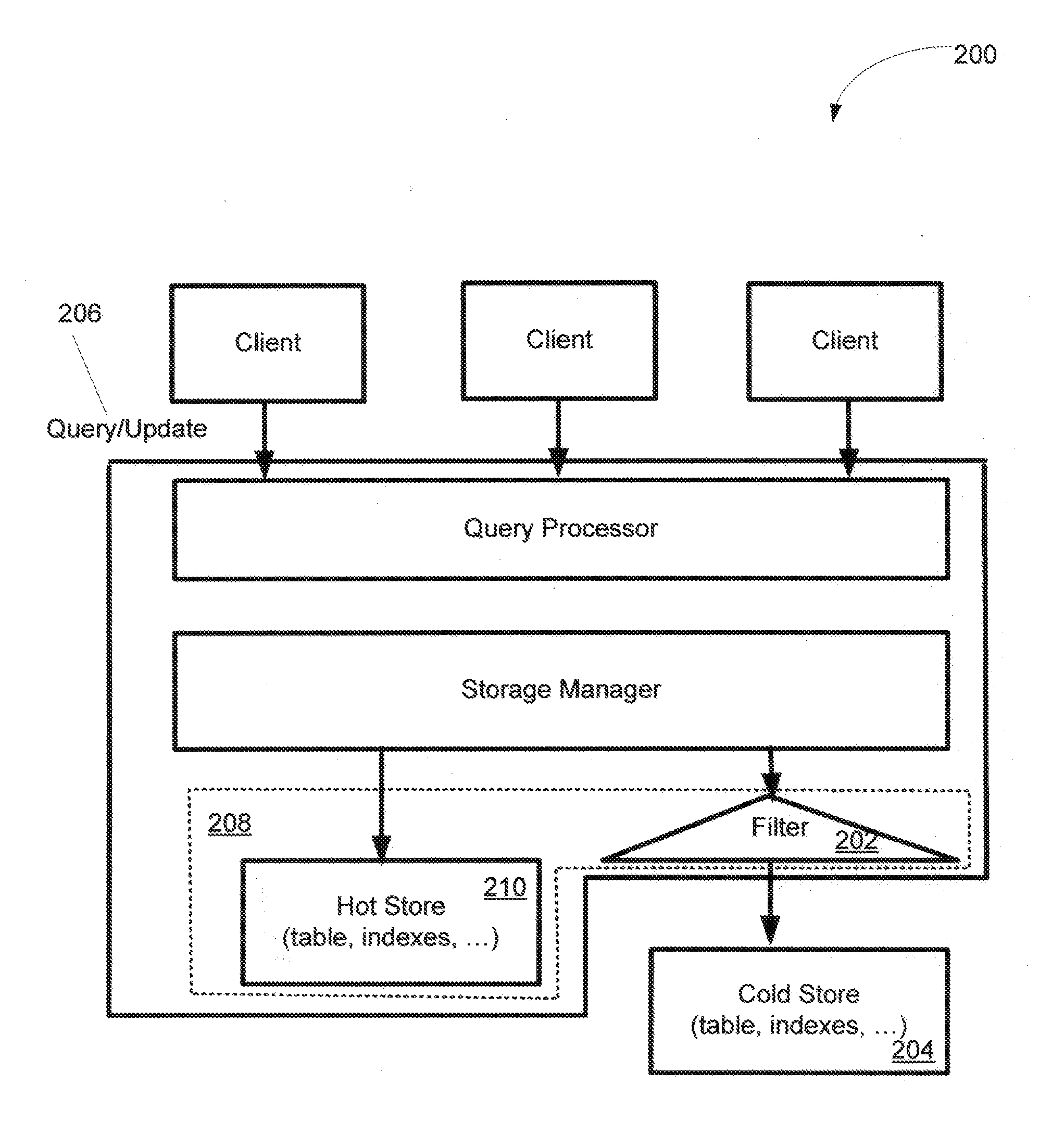
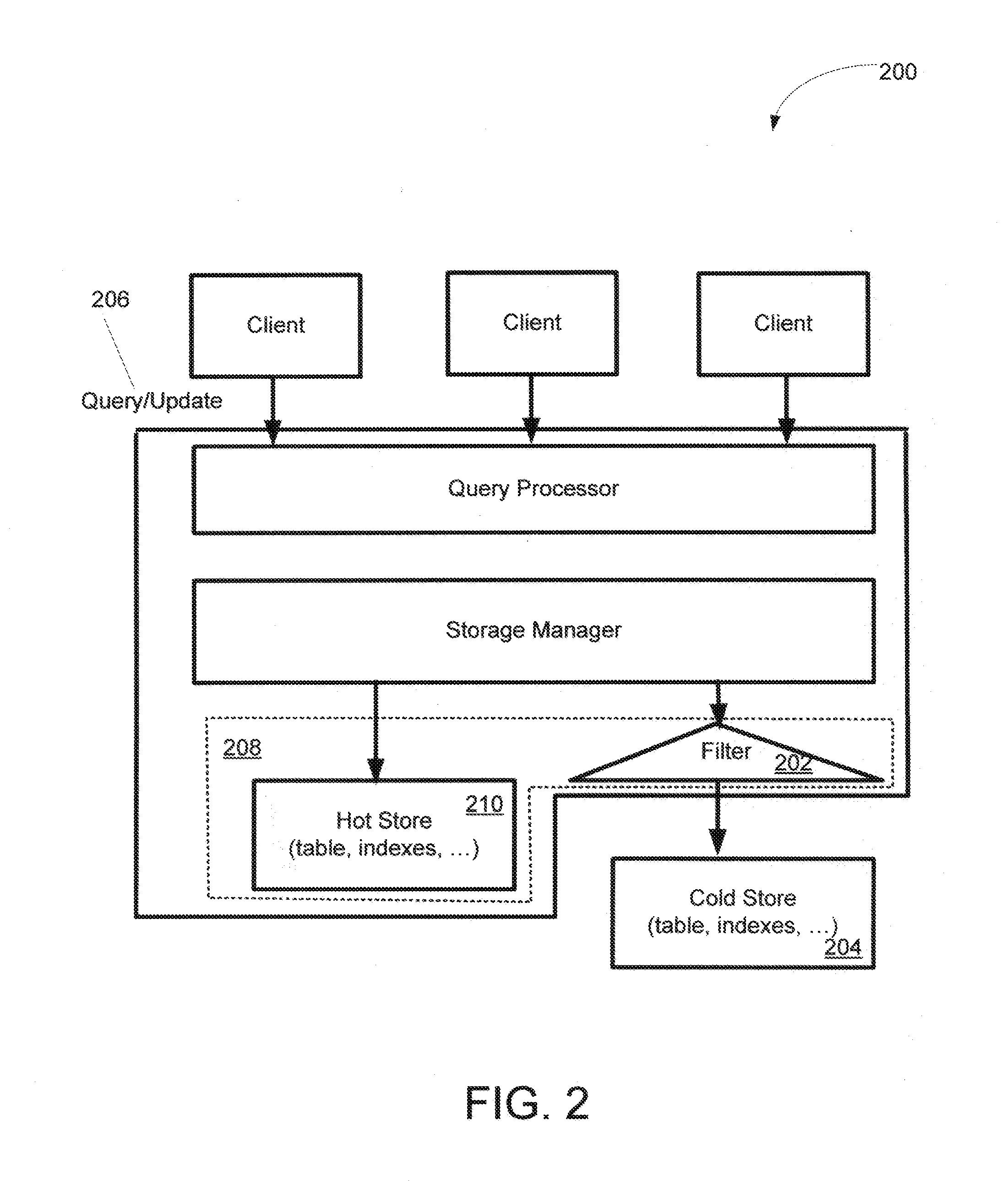
Access to the (cold) store 204 is assumed to be expensive even if it is only to find out that the store contains no relevant information for a query or update operation.

Bloom filters, for instance, are not adaptive and their precision deteriorates when many records have migrated between the hot and cold stores.

1) Correctness: The filter should not generate false negatives. That is, if the filter returns false for a query or data update, then it should be certain that the cold store contains no relevant records.

2) Precision: The number of false positives should be minimized. A false positive is a query or update for which the filter returns true even though the cold store contains no relevant records. False positives do not jeopardize the correctness of the query results, but they hurt performance.

3) Space efficiency: The filter should ideally be located in the hot store to guarantee efficient access to the filter. As space in the hot store is expensive, minimizing the space occupied by the filter is critical to be cost effective.

4) Graceful degradation: A direct consequence of the space efficiency requirement is that the precision of a filter should grow and degrade with its space budget. Even a tiny filter should be useful and filter out the most common queries.

5) Speed: Filtering is preferably much faster than access to the cold store. The cost of filtering ideally is in the same order as processing a query in the hot store: Most queries are expected to be hot only queries and almost all queries (except for primary key lookups in the hot store) involve a filtering step. That is why the filter ideally lives in the hot store.

6) Robustness: By design, most queries and updates involve hot data only. Therefore typically both the data distribution and the query distribution are heavily skewed. The filter should be designed to work well in such situations. Furthermore, the filter preferably adapts whenever the workload changes and / or data is migrated back and forth from the cold to the hot data store.

7) Generality: The filter preferably should not make any assumptions about the partitioning scheme used to classify records as hot or cold. It should support partitioning at the record level, the finest possible granularity. Furthermore, the filter should support any kind of query and update: that is, both equality and range predicates.

Unfortunately, Bloom filters are not a good match for range queries.

Furthermore, they do not exploit skew in the data and workload and do not adapt to changes in the data and workload.

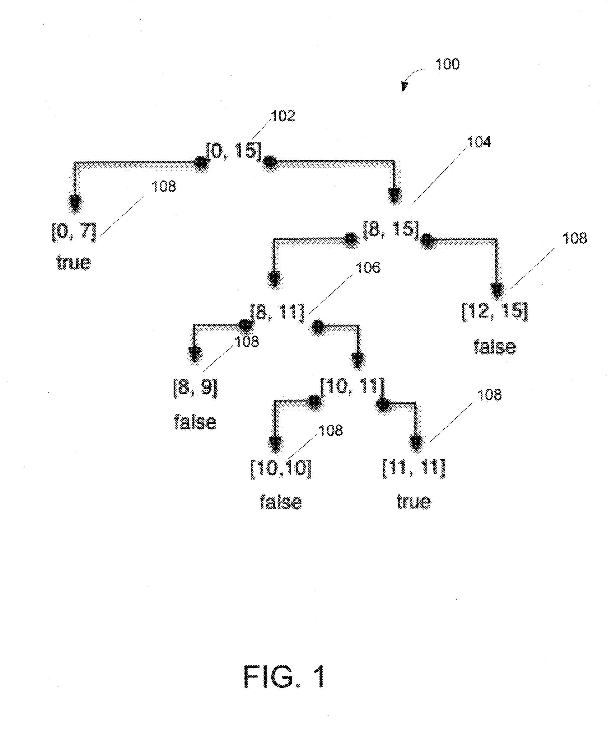
False positives may arise in a number of situations: Most importantly, an adaptive range filter cannot precisely represent all the keys of the cold store if there is a limited space budget.

As a result, the adaptive range filter of FIG. 6 results in a false positive for the query [4,4].

1) Space: The root node of the adaptive range filter need not store the boundaries of the range it represents. These boundaries are implicitly stored in the B-tree.

2) Space: The technique saves the bits to encode the upper levels of the big adaptive range. For instance, the four bits to represent nodes [0,15] and [8,15] in the big adaptive range filter of FIG. 6 are not needed and the three adaptive range filters of FIG. 6 can be represented with a total of 9 bits (instead of 13 bits).

3) Time: The technique saves the cost to navigate the first levels of the adaptive range filter. In other words, while traversing the B-tree, the technique implicitly also navigates through the top levels of the adaptive range filter.

If space is limited, then the technique needs to de-escalate the adaptive range filter, thereby gaining space and losing precision.

However, perfection is not necessary and the technique can often achieve very good results (few false positives) by exploiting skew in the workload associated with querying or updating the stored data.

Fortunately, unlike insertions, deletions in the cold store cannot result in incorrect adaptive range filters: the worst that can happen is that they result in inefficiencies caused by false positives.

1) Explore the Data: A table in the cold store is scanned. From the results, a perfect adaptive range filter which accurately models all gaps in the cold store is constructed. Such a perfect adaptive range filter, for instance, would escalate Node [0,7] in FIG. 6 to capture that the cold store contains no keys that match 4 and 7. This adaptive range filter is likely to exceed the space budget, but that is typically tolerable in the training phase. (The adaptive range filter is trimmed to fit its space budget in step 3 below.)

2) Explore the Workload: A series of example queries and updates which are representative for the query and update workload are run. The purpose of this step is to make sure that the adaptive range filter learns the query / update distribution. As part of this step of the training phase, usage counters are kept at all the leaves of the perfect adaptive range filter indicating how often each leaf was involved in a query or update.

3) Meet Space Constraints: The adaptive range filter is trimmed by iteratively selecting the leaf with the lowest usage counter as a victim for replacement (as part of a de-escalation) until the adaptive range filter fits into the space budget. At this point, all of the usage counters are discarded and more space-efficient usage statistics such as used bits for a clock strategy or even no statistics at all are kept.

Images