[0041] The technical solutions in the embodiments of the present invention will be clearly and completely described below in conjunction with the accompanying drawings in the embodiments of the present invention. Obviously, the described embodiments are only a part of the embodiments of the present invention, rather than all the embodiments. Based on the embodiments of the present invention, all other embodiments obtained by those of ordinary skill in the art without creative work shall fall within the protection scope of the present invention. In addition, the protection scope of the present invention should not be limited to the following specific steps or specific parameters.
[0042] The method of suppressing reverse time migration low frequency noise of the present invention is based on the following research:
[0043] (1) Source normalization The cross-correlation imaging conditions are normalized under the original cross-correlation imaging conditions. The cross-correlation imaging conditions can be expressed as follows:
[0044] M RS i , j = ∫ W S i , j t * W R i , j t dt
[0045] Where Is the source wave field, It is the wave field of the detection point. Among them, i, j are the coordinates in the x and z directions, the unit is m, t is the different time of the wave field, the unit is s, and the imaging value is the accumulation of the correlation results at all times.
[0046] (2) The amplitude preservation effect of the cross-correlation imaging condition itself is poor, and the normalized imaging condition of the seismic source has more amplitude fidelity compared with it, and its form is as follows:
[0047] M RS i , j = ∫ W S i , j t * W R i , j t dt ∫ W S i , j t * W S i , j t dt
[0048] (3) Compared with the cross-correlation imaging conditions, the source normalized cross-correlation imaging conditions can attenuate the shallow energy and increase the deep energy to a certain extent.
[0049] The normalized cross-correlation imaging conditions of the seismic source will inevitably introduce low-frequency noise during the imaging process, which brings a certain degree of interference to the imaging results. Laplacian filtering is a commonly used filtering method to remove low-frequency noise. It directly processes the imaging volume and has an obvious effect on removing low-frequency noise.
[0050] The Laplacian can be expressed as:
[0051] ▿ 2 = ∂ x 2 + ∂ z 2
[0052] Where Denote the second-order partial derivatives of x and z respectively.
[0053] It can be expressed in the wavenumber domain as:
[0054] FFT ( ▿ 2 ) = - ( k x 2 + k z 2 ) = - | k I → | 2
[0055] Where Is the wave number vector, there are FFT stands for Fourier transform.
[0056] From the law of cosines:
[0057] | k I → | 2 = | k R → | 2 + | k S → | 2 - 2 | k R → | | k S → | cos ( π - 2 θ ) = 4 ω 2 v 2 cos 2 θ
[0058] In the formula, θ is the incident angle, They are the wave number vectors of the wave field of the detector and the wave field of the seismic source.
[0059] After the imaging data volume is filtered by Laplacian, there is still a certain amount of noise residue, and non-local mean filtering can filter out the noise well. The principle of non-local mean filtering is as follows:
[0060] An imaging result I with noise can be expressed as follows:
[0061] I=U+N
[0062] In the formula, U is the imaging result without noise, and N is noise.
[0063] For any position m in the imaging result, the imaging result after denoising It can be expressed as:
[0064] I ^ ( m ) = X k w ( m , k ) I ( k )
[0065] In the formula, w(m,k) is the similarity of imaging values between m and k, which satisfies 0≤w(m,k)≤1 and Σ k w(m,k)=1. Among them, each m has a similarity coefficient related to k. In order to quantify the similarity, define N m Is a window centered on m. To calculate N m And N k The similarity between is expressed by Gaussian weighted Euclidean distance:
[0066] D 2 ( m , k ) = | | I ( N m ) - I ( N k ) | | 2 , a 2 = X l nl [ G u ( l ) ( I ( N m ( l ) ) - I ( N k ( l ) ) ) ] 2
[0067] Where Is the square of the Gaussian weighted Euclidean distance, G u Is a Gaussian function, and its form is:
[0068] G u ( x , y ) = exp ( - ( x - x 0 ) 2 + ( y - y 0 ) 2 2 u )
[0069] Where x 0 , Y 0 Is the center of the Gaussian function, where x and y correspond to the l term in the above formula, and u is the deviation parameter.
[0070] N m And N k The similarity coefficient between can be expressed as:
[0071] w ( m , k ) = 1 Z ( m ) exp ( - D 2 ( m , k ) h 2 ) - - - ( * )
[0072] among them, Is the regularization coefficient to ensure that Σ k w(m,k)=1.
[0073] The invention will be further elaborated below. The invention is not limited to Walkaway VSP reverse time migration, it is also applicable to ground seismic reverse time migration, and it can process actual data and has a wide range of adaptability.
[0074] The method for suppressing reverse time offset low-frequency noise of the present invention includes the following steps:
[0075] 1) Deploy geophones at regular intervals in the vertical direction of the well, set shot lines across the wellhead on the surface, and shot points at equal intervals, artificially excite seismic waves, and record the Walkaway VSP seismic signals received in the well on tape;
[0076] 2) Read seismic records from magnetic tapes, do conventional noise suppression, deconvolution, wavefield separation and velocity analysis, etc., to obtain preprocessed shot records and velocity models;
[0077] 3) Read the Walkway VSP shot record, perform Fourier transform to obtain the amplitude spectrum of the shot record, analyze the main frequency of the shot record, denote it as f p , The unit is Hz, the seismic wavelet is calculated according to the following formula:
[0078] f ( t ) = [ 1 - 2 ( π f p t ) 2 ] e - ( π f p t ) 2 - - - ( 1 )
[0079] 4) Read the velocity model, use the wavelet obtained in step 3) as the source wavelet, and use the two-way wave equation to calculate the forward wave field;
[0080] 5) Read the Walkway VSP shot record and velocity model, use the shot record as input, and use the two-way wave equation to calculate the back propagation wave field;
[0081] 6) Step 4) and step 5) start looping from the first shot, do data processing for each shot, and use source normalized cross-correlation imaging conditions to image the forward and reverse wave fields;
[0082] 7) Laplacian filtering the imaging data volume to obtain filtered seismic data;
[0083] 8) Read the velocity model and find the similarity coefficients required by the non-local mean filtering calculation process;
[0084] 9) Perform non-local mean filter processing on the filtered seismic data to obtain the final output data. The result data will indicate the division of geological horizons and determine the interpretation plan for the micro-fault system, which is also used for reservoir prediction and oil and gas-benefit District identification.
[0085] Preferably, the seismic source wavelet required for the Walkaway VSP reverse time migration used in step 3) is designed as the Lake wavelet.
[0086] Preferably, the sound wave equation used in the forward and reverse propagation of the wave field in step 4) and step 5) can be written as:
[0087] ∂ 2 w ∂ t 2 = v 2 ( ∂ 2 w ∂ x 2 + ∂ 2 w ∂ z 2 )
[0088] Where: w is the wave field value, which is a function of space coordinates (x, y, z) and time t, and v is the speed of the corresponding space position, in m/s.
[0089] Step 4) After reading the velocity model v, set the spatial grid step size in the x and z directions Δx=Δz=Δd, and use the following formula to determine the time sampling step.
[0090] vΔt Δd 1 / 2 X m = 1 N 1 b 2 m - 1
[0091] In the formula, N is the difference order, N 1 Is the largest odd number less than N; Δt is the time step, and b is the difference coefficient.
[0092] In step 6), the source wave field and the wave field of the detector are cross-correlated at each time, and the correlation results at all times are accumulated, and compared with the accumulated value of the autocorrelation of the source wave field at all times. The calculation formula for normalized cross-correlation imaging conditions of seismic sources:
[0093] M RS i , j = ∫ W S i , j t * W R i , j t dt ∫ W S i , j t * W S i , j t dt
[0094] Where Is the source wave field, Is the wave field of the detection point, i and j are the coordinates in the x and z directions respectively, the unit is m, t is the time, and the unit is s. It is to first cross-correlate the seismic source wave field and the wave field of the detection point at each time, and then autocorrelate the seismic source wave field, and finally compare the accumulated cross-correlation results at all times with the accumulated auto-correlation results at all times.
[0095] The Laplacian filtering of step 7) performs filtering processing equivalent to the angle domain on the imaging data volume of step 6).
[0096] Step 8) Non-local mean filtering first obtains similarity coefficients for the velocity model, and performs non-local mean filtering on the data volume after Laplace filtering to suppress residual noise in the seismic migration data.
[0097] In the following, the invention will be further schematically illustrated in conjunction with the drawings and examples.
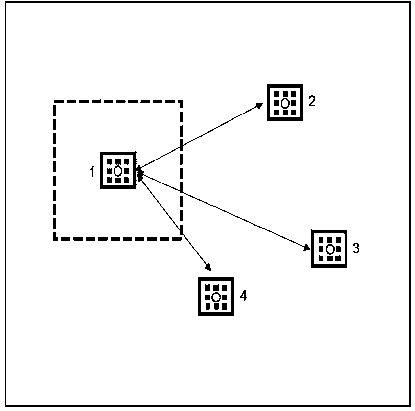
[0098] Reference attachment figure 1 , The figure shows the calculation of the similarity coefficient between the window centered on the dot in box 1 and the window centered on the surrounding points. For example, to calculate the similarity coefficient between the center point of box 1 and the center point of box 2, first determine the window The size is the size of the data included with the point as the center, and then the Gauss Euclidean distance is calculated for the data between the 1 frame and the 2 frame, and finally the similarity coefficient between the center points of the two frames is obtained. Non-local mean filtering originally calculates similarity coefficients for the whole world, such as calculating the similarity coefficients between the center point of frame 1 and all other points in the imaging body, but this will generate a large amount of calculation, so it is only centered on the center point of frame 1. The similarity coefficient is calculated for all points within the dashed border.
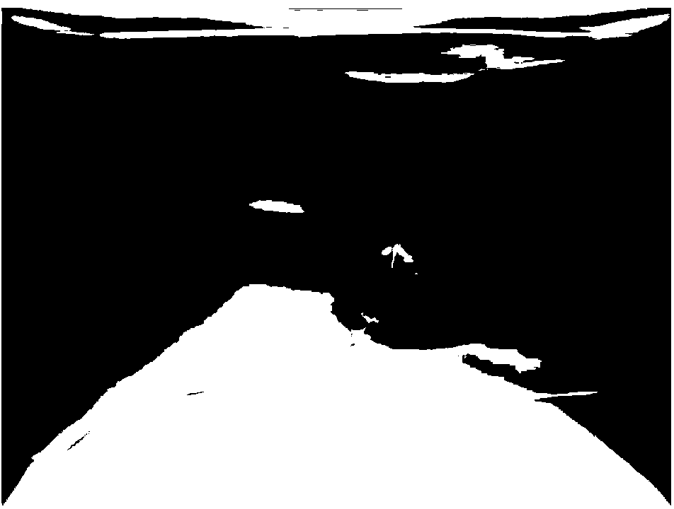
[0099] Reference attachment figure 2 It is the result of Walkaway VSP reverse time migration cross-correlation imaging. It can be seen that there is obvious low-frequency noise, which affects the final imaging effect.
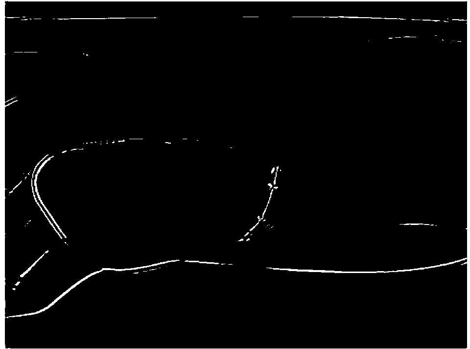
[0100] Reference attachment image 3 For the imaging volume after Laplacian filtering, it can be seen that low-frequency noise is better suppressed, indicating that Laplacian filtering has a relatively obvious denoising effect.
[0101] Reference attachment Figure 4 It is the velocity model of the imaging body. In order to actually verify the effect of non-local mean filtering, the actual velocity model is smoothed and used as the input graph for non-local mean filtering to obtain similar coefficients.
[0102] Reference attachment Figure 5 It is the imaging volume after non-local mean filtering. It can be seen that the noise is significantly reduced and the seismic imaging is clearer.
[0103] Reference attachment Image 6 with Figure 7 Respectively are image 3 with Figure 5 The local zoomed-in comparison map of, compared with the position shown by the white arrow, it can be seen that after non-local mean filtering, the noise of the imaging data is further suppressed, and the local structure is clearer.
[0104] Obviously, the above-mentioned embodiments are only examples to clearly illustrate the present invention, and are not intended to limit the embodiments. For those of ordinary skill in the art, on the basis of the above description, other changes or changes in different forms can be made, and it is not necessary and impossible to list all the implementation manners here. Obvious changes or alterations derived from this are still within the protection scope of the invention.