[0019] In order to facilitate the understanding and implementation of the present invention by those of ordinary skill in the art, the present invention will be further described in detail with reference to the accompanying drawings and embodiments. It should be understood that the implementation examples described here are only used to illustrate and explain the present invention, and are not intended to limit this invention.
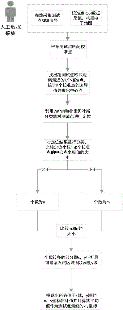
[0020] Please see figure 1 , A WiFi indoor positioning method based on domain clustering provided by the present invention includes the following steps:
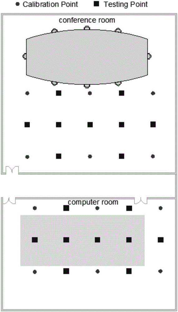
[0021] Step 1: Select 6 calibration points in two different indoor environments (see figure 2 ), collect WiFi signal strength information at the calibration point for a duration of 2 min; associate the signal strength information with the position information of the calibration point to form a location fingerprint to obtain a location fingerprint library;
[0022] Step 2: Collect WiFi signal strength information of test points (x, y) (9 test points, see for details figure 2 ), the WiFi signal strength information of the test point is pre-matched with the location fingerprint library, and the Euclidean distance between the calibration point and the test point is used to find the K adjacent calibration points closest to the test point; the boundary values of the K adjacent calibration points are counted and combined Find the center point;
[0023] In this embodiment, the number of adjacent calibration points is set to 4. At the same time, the coordinate boundary values of the four adjacent calibration points are recorded as and
[0024] Step 3: Use WKNN or Naive Bayes classifier to locate the test points; if there are a total of m APs observed by the calibration point and the test point, the possible positions of the m test points can be obtained;
[0025] To identify the approximate area of the test point, the simple AP visibility principle can be applied to achieve this goal. Generally speaking, the set of APs visible in the room-level sub-areas is different, so the area with the largest number of APs that can be observed with the test point is the most likely area of the test point, that is, the approximate area. The AP that can be observed by all test points and calibration points in the approximate area is recorded as AP 1 , AP 2 ,...,AP m.
[0026] The concrete realization principle of WKNN method and Naive Bayes method:
[0027] Select k APs for position estimation, so the RSS vector of the j-th calibration point is:
[0028]
[0029] The distance of the multi-dimensional signal space between the calibration point and the positioning point It can be expressed as Euclidean distance:
[0030]
[0031] among them, Indicates the RSS observation value of the i-th AP of the test point;
[0032] Select the K calibration points with the shortest distance to estimate the position of the test point. The difference between WKNN and Naive Bayes classifier is the weight calculation;
[0033] WKNN usually uses the inverse distance weighting:
[0034]
[0035] Therefore, the location of the test point can be calculated by the following formula:
[0036]
[0037] among them Indicates the estimated value of the two-dimensional coordinate of the test point, Indicates the coordinates of the j-th calibration point;
[0038] Suppose the RSS observation vector of the test point is and Represents the location of the j-th calibration point, then the naive Bayes classifier uses the posterior probability Measure the probability that the test point appears at the jth calibration point; using Bayesian theory, the posterior probability It can be expressed in the following form:
[0039]
[0040] among them Represents RSS t The conditional probability is stored in the fingerprint library at the offline stage. Is the same constant;
[0041] Similar to WKNN, will As the weight of the j-th calibration point, the position estimation formula of the naive Bayes classifier of the test point is as follows:
[0042]
[0043] Step 4: Determine the final location of the test point Its concrete realization includes the following sub-steps:
[0044] Step 4.1: Sort the x and y coordinates of the possible positions of m test points respectively;
[0045] Step 4.2: Use the x-coordinates of m estimated positions Divided into two parts, of which Indicates the largest x-coordinate value in the possible position of the test point; Indicates the smallest x-coordinate value in the possible position of the test point;
[0046] Step 4.3: Calculate less than And greater than The number of x-coordinates, the area where the x-coordinates are most likely to fall, becomes the x-domain;
[0047] Step 4.4: Pick out all the estimated x-coordinates in the x-domain and use the following formula to calculate the final x-coordinate of the test point
[0048]
[0049] Where k x Represents the number of coordinates in the x domain, Represents the coordinate estimation belonging to the x domain;
[0050] Step 4.5: Use the principles of steps 4.1-4.1 to calculate the final estimated value of the y coordinate of the test point
[0051] Step 4.5: Get the final location of the test point
[0052] The real location (x, y) and estimated location of the test point The error err can be calculated as follows:
[0053]
[0054] The experimental results of this embodiment are as follows. The accuracy comparison results of the WKNN algorithm and the WKNN-DCL algorithm are shown in Table 1, and the accuracy comparison results of the Naive Bayes algorithm and the Naive Bayes-DCL algorithm are shown in Table 2. The WKNN algorithm and WKNN- The comparison results of the stability of the DCL algorithm are shown in Table 3, and the comparison results of the stability of the Naive Bayes algorithm and the Naive Bayes-DCL algorithm are shown in Table 4:
[0055] Table 1 Comparison of accuracy between WKNN algorithm and WKNN-DCL algorithm
[0056]
[0057]
[0058] Table 2 Accuracy comparison between Naive Bayes algorithm and Naive Bayes-DCL algorithm
[0059]
[0060] Table 3 Comparison of WKNN algorithm and WKNN-DCL algorithm stability
[0061]
[0062]
[0063] Table 4 Comparison of the stability of the naive Bayes algorithm and the naive Bayes-DCL algorithm
[0064]
[0065] Experiments were conducted in the area of two rooms to evaluate the performance of the proposed new method. Room 1 is a computer room with personnel activities, the size is about 72m 2 (10m×7.2m). Room 2 is a conference room with no people moving around, the size is about 110m 2 (10m×11m). A total of 12 calibration points and 18 test points were collected. The space between adjacent points is 2m. The physical locations of calibration points and test points are as figure 2 Shown.
[0066] Two typical methods, WKNN and Naive Bayes classifier are selected for comparative analysis with DCL. The AP selection of WKNN and Naive Bayes classifier adopts an intelligent AP selection strategy based on joint information gain, and the number of AP subsets is set to 4-8 respectively. Implement DCL based on WKNN (WKNN-DCL) and DCL based on Naive Bayes classifier (NBC-DCL) respectively. Table 1 compares the mean, standard deviation and maximum error of the position estimation errors of WKNN and WKNN-DCL two different strategies. Table 2 compares the mean, standard deviation, and maximum error of the position estimation error of two different strategies of Naive Bayes classifier and NBC-DCL. It can be seen from Table 1 and Table 2 that the positioning results of the classic WKNN method and the naive Bayes classifier are both affected by the number of AP subsets, and it is difficult to find the difference between the mean and maximum error and the number of AP subsets. Show relationship. Therefore, these two methods need to carefully deal with the issue of selecting the number of APs. In Table 1 and Table 2, the mean error of WKNN-DCL is smaller than that of the WKNN method with different AP numbers, and the mean error of NBC-DCL is also smaller than the naive Bayes classifier with different AP numbers. At the same time, the maximum error of NBC-DCL is also much smaller than the results calculated by other naive Bayes classifiers, and the error standard deviation of NBC-DCL is also the smallest. However, there are some abnormalities in the comparison of WKNN-DCL. The error standard deviation of WKNN-DCL is not the smallest, and its maximum error is the largest.
[0067] image 3 with Figure 4 The cumulative distribution function graph (CDF) of different positioning strategies is shown. Such as image 3 As shown, when the error threshold is between 2m and 4m, the CDF curve of WKNN-DCL is higher than that of the classic WKNN method, that is, the probability that the error is less than the threshold is higher. This phenomenon is Figure 4 It is more obvious that the CDF curve of NBC-DCL is higher than the naive Bayes classifier in the entire error range. Table 3 and Table 4 show the statistical percentages of accuracy within 1.5m, 2.5m and 3.5m. The error of WKNN-DCL less than 1.5m accounts for 61%, which is much larger than the classic WKNN method. Although the percentage of accuracy of WKNN-DCL at 2.5m is worse than that of some WKNN methods, the percentage of accuracy of WKNN-DCL less than 3.5m is 89%, which is about 6% higher than the best WKNN method. The accuracy of the 1.5m tolerance of NBC-DCL is 44% and the accuracy of 3.5m is 83%, which is much better than the naive Bayes classifier.
[0068] It should be understood that the parts not elaborated in this specification belong to the prior art.
[0069] It should be understood that the above description of the preferred embodiments is more detailed and should not be regarded as a limitation of the scope of protection of the present invention. Those of ordinary skill in the art, under the enlightenment of the present invention, do not depart from the claims of the present invention. In the case of the scope of protection, alternatives or modifications may be made, and all fall within the scope of protection of the present invention. The scope of protection of the present invention shall be subject to the appended claims.