Method for establishing model for obtaining glomerular filtration rate and application

[0027] In order to make the above-mentioned objects, features and advantages of the present invention more obvious and understandable, the specific embodiments of the present invention will be described in detail below with reference to the accompanying drawings. In the following description, many specific details are explained in order to fully understand the present invention. However, the present invention can be implemented in many other ways different from those described herein, and those skilled in the art can make similar improvements without departing from the connotation of the present invention. Therefore, the present invention is not limited by the specific implementation disclosed below.

[0028] The patient data collected in this embodiment comes from the Third Xiangya Hospital (TXH) of Central South University (TXH) and the Second Xiangya Hospital (SXH) of Central South University in central China (Changsha City, Hunan Province), and the First Affiliated Hospital of Xinjiang Medical University (FXH) Patients who have undergone 99mTc-DTPA renal dynamic imaging have been approved by the local ethics committee. Exclude patients younger than 18 years old or lack of basic creatinine value or mGFR value, or patients on dialysis, or have used drugs that affect creatinine or basic creatinine in the 10 days before the kidney map> 700μmol/L patients. The collected data include demographic data: height, age, weight, gender; inspection: 99mTc-DTPA renal dynamic imaging measurement; creatinine, blood routine, and other blood and urine biochemical indicators. In the end, 2472 inpatients in TXH hospital were randomly allocated according to 7:3, of which 70% (1730 inpatients) were used as training set for modeling, and the remaining 30% (742 inpatients) were used as validation set for internal verification; According to the inclusion and exclusion criteria, 300 outpatients were selected as the validation set for internal verification.

[0029] This specific embodiment proposes a method for establishing a model for obtaining glomerular filtration rate of the Chinese population, including the steps:

[0030] S0. Log conversion of the known glomerular filtration rate of 1648 patients.

[0031] S1. Perform log conversion on multiple candidate independent variables corresponding to the glomerular filtration rate after log conversion, and use least squares linear regression to perform univariate analysis on multiple candidate independent variables after log conversion to P <0.010 is the standard, select P For the first independent variable <0.010, P represents a parameter for testing the significance level of the first independent variable.

[0032] It should be noted that multiple candidate independent variables include age, gender, cystatin C, α1 microglobulin, β2 microglobulin, carbon dioxide binding capacity, chlorine determination, anion gap, alanine aminotransferase, and Tianmen Aspartate aminotransferase, total bilirubin, total protein, albumin ratio, direct bilirubin, globulin, total bile acid, pH, high-density lipoprotein cholesterol, low-density lipoprotein cholesterol, triglycerides, high Density cholesterol ratioTotal cholesterol, total cholesterol, albumin, blood glucose, prothrombin time, activated partial thromboplastin time, thrombin time, red blood cells, white blood cells, hemoglobin, hematocrit, average red blood cell volume, average red blood cell hemoglobin content, average Red blood cell hemoglobin concentration, lymphocyte absolute value, neutrophil absolute value, neutrophil percentage, monocyte absolute value, monocyte percentage, eosinophil absolute value, lymphocyte percentage, eosinophil percentage, basophil Absolute cell value, percentage of basophils, platelet variables, platelet distribution width, platelet specific volume, average platelet volume, red blood cell distribution width, serum potassium ion concentration, serum calcium ion concentration and serum sodium ion concentration. A plurality of the first independent variables include gender, age, height, weight, creatinine, chlorine, aspartate aminotransferase, total protein, globulin, average red blood cell hemoglobin concentration, total bile acid, red blood cell, average red blood cell volume, Percentage of monocytes and uric acid.

[0033] S2. Use multiple linear regression modeling for a plurality of the first independent variables to perform multi-element analysis, and simplify the number of the first independent variables to establish a first model. The functional expression of the first model is GFR=94047.95 ×0.8892828 a ×N -0.22630 ×C -0.52474 ×L -0.92495 ×H 0.28309; Among them, GFR means glomerular filtration rate; a is a coefficient related to gender, when the gender is male, a is 0, when the gender is female, a is 1; N is age; C is the concentration of creatinine; L represents the concentration of chloride ions; H represents the concentration of red blood cells. Wherein, simplifying the number of the first independent variables to establish a first model specifically includes using R 2 , AdjustedR 2 And AIC is the judgment criterion to preliminarily screen the second independent variable from the first independent variable, and use the second independent variable according to R 2 Sort from largest to smallest, filter out the top 5 second independent variables, and build the first model.

[0034] It should be noted that R 2 With adjustedR 2 Both represent the coefficient of determination, which refers to the proportion of the selected independent variable that can explain the dependent variable, and is used to evaluate the pros and cons of the regression line fitting. The larger the value, the better the fit. While adjustedR 2 After removing the influence of the number of independent variables, the explanatory power of the regression equation can be evaluated more accurately. AIC is the abbreviation of Akaike Information Criterion, which stands for "Akaike Information Criterion". It is a standard to weigh the complexity of the estimated model and the goodness of the fitted data. Usually the model with the smallest AIC is selected as the best model, so that the smallest AIC, R 2 With adjustedR 2 The largest second argument.

[0035] S3. Simplify the first model to obtain a second model, and the function expression of the second model is GFR=1363.868×0.8823822 a ×N 0.22910 ×C -0.53755 ×H 0.28458; Among them, GFR means glomerular filtration rate; a is a coefficient related to gender, when the gender is male, a is 0, when the gender is female, a is 1; N is age; C is the concentration of creatinine; H represents the concentration of red blood cells. Although the chloride ion concentration variable is statistically significant, the important role of chloride ion level on GFR cannot be explained clinically at this stage. Therefore, combined with the clinical significance, the second independent variable of chloride ion concentration is removed at this stage.

[0036] S4. Simplify the second model to obtain a third model, and the function expression of the third model is GFR=2374.78×0.8526126 a ×N -0.25011 ×C -0.54753; Among them, GFR represents the glomerular filtration rate; a is a coefficient related to gender, when the gender is male, a is 0, when the gender is female, a is 1; N represents age; C represents the concentration of creatinine. Although the red blood cell concentration variable is statistically significant, if the formula is imported as the second independent variable, in actual use, patients who have not tested red blood cells cannot use this formula. In order to facilitate clinical application, the second independent variable of red blood cell concentration is removed. The result of the training set is GFR≤60 group: P 30 =0.576; 60 30 =0.913; GFR> Group 90: P 30 =0.843, the training set adopts the third model to obtain P of glomerular filtration rate 30 = 79.5%, higher than the P specified in the guidelines 30 75%, with clinical significance; for different levels of GFR, the new formula of P 30 Are greater than the P of other existing eGFR formulas 30 Level (GFR≤60, P 30 Although lower than 75%, it is still higher than other existing formulas). The result of the validation set is GFR≤60 group: P 30 = 57.0%, 60 30 = 92.7%, GFR> Group 90: P 30 = 81.5%, the training set adopts the third model to obtain P of GFR 30 = 78.7%. The results of the validation set are basically the same as those of the training set. It illustrates the stability and accuracy of the third model to obtain GFR.

[0037] It should be noted that, according to reports, the daily GFR variability of an individual is 17%, so it is stipulated that 15%-30% is a reasonable range of mGFR variability. According to the 2002 K/DOQI guidelines, use P 30 It represents the variation of the estimated value eGFR within the range of the actual measured value mGFR ±30%. P 30 Reflects the ratio of error (the difference between eGFR and mGFR) to the test result (mGFR) (1±30%). It has good consistency and stability and is an important indicator for evaluating the accuracy of the formula .

[0038] The 2002 K/DOQI guidelines point out that the P of the eGFR formula 30 = 75% is the minimum standard for effective clinical decision-making. Therefore, the P of the eGFR formula 30 75% indicates that the accuracy of the formula meets the guideline standard, has clinical significance, and can be applied to the clinic.

[0039] In this specific embodiment, before performing log conversion on multiple candidate independent variables corresponding to the glomerular filtration rate after log conversion, it also includes performing "cubic spline processing" or "without any processing" on all candidate independent variables. ", by transforming the candidate independent variables in different forms to reflect the multiplicative relationship with the dependent variable, and stabilize the variance of the candidate independent variable within the GFR range. The results show that "log transformation" has the best effect. Therefore, "log transformation" is selected as the basic form of the independent variable import model.

[0040] The specific processing results are as follows:

[0041] 1. Gender:

[0042] adjustedR 2 =0.001724, P <0.001.

[0043] 2. Age: Try the following six situations:

[0044] No treatment of age, directly import the model: adjusted R 2 =0.05086, P <0.001;

[0045] Nothing is done for age, but the cubic spline form (3 nodes) of age is imported into the model: adjustedR 2 =0.05557, P <0.001;

[0046] Nothing is done for age, but the cubic spline form (5 nodes) of age is imported into the model: adjustedR 2 =0.0634, P <0.001;

[0047] Perform log transformation on age and directly import the model: adjusted R 2 =0.04472, P <0.001;

[0048] Perform log transformation on age and import the cubic spline form (3 nodes) of age into the model: adjustedR 2 =0.05442, P <0.001;

[0049] Perform log transformation on age, and import the cubic spline form (5 nodes) of age into the model: adjustedR 2 =0.05667, P <0.001.

[0050] 3. Height: Try the following six situations:

[0051] Do not do any processing on the height, directly import the model: adjustedR 2 = -0.0002757, P = 0.859;

[0052] Nothing is done on the height, but the cubic spline form (3 nodes) of the height is imported into the model: adjustedR 2 =-0.0005599, P=0.983;

[0053] Nothing is done on the height, but the cubic spline form (5 nodes) of the height is imported into the model: adjustedR 2 =0.001871, P =0.0318;

[0054] Perform log transformation on height and directly import the model: adjusted R 2 = -0.000186, P = 0.558;

[0055] Perform log transformation on height, and import the cubic spline form (3 nodes) of height into the model: adjustedR 2 = -0.0002775, P = 0.8733;

[0056] Perform log transformation on height, and import the cubic spline form (5 nodes) of height into the model: adjustedR 2 =0.001814, P=0.346.

[0057] 4. Weight: Try the following six situations:

[0058] Do not do any processing on the weight, directly import the model: adjustedR 2 = -0.0002724, P = 0.8353;

[0059] Nothing is done on the weight, but the cubic spline form (3 nodes) of the weight is imported into the model: adjustedR 2 = 0.0001307, P = 0.293;

[0060] Nothing is done on the weight, but the cubic spline form (5 nodes) of the weight is imported into the model: adjustedR 2 = -0.0002001, P = 0.5094;

[0061] Perform log transformation on the weight and directly import the model: adjustedR 2 = -0.0002797, P = 0.914;

[0062] Perform log transformation on the weight, and import the cubic spline form (3 nodes) of the weight into the model: adjustedR 2 = 0.0002654, P = 0.2309;

[0063] Perform log transformation on the weight, and import the cubic spline form (5 nodes) of the weight into the model: adjustedR 2 = -0.0001354, P = 0.4743.

[0064] 5. Creatinine: Try the following six situations:

[0065] No treatment for creatinine, directly import the model: adjusted R 2 =0.506, P <0.001;

[0066] No treatment is done on creatinine, but the cubic spline form (3 nodes) of creatinine is imported into the model: adjustedR 2 = 0.6891, P <0.001;

[0067] No treatment for creatinine, but the cubic spline form (5 nodes) of creatinine is imported into the model: adjustedR 2 = 0.6897, P <0.001;

[0068] Perform log transformation on creatinine and directly import the model: adjusted R 2 = 0.6759, P <0.001;

[0069] Perform log transformation on creatinine, and import the cubic spline form (3 nodes) of creatinine into the model: adjustedR 2 = 0.6766, P <0.001;

[0070] Perform log transformation on creatinine and import the cubic spline form (5 nodes) of creatinine into the model: adjustedR 2 = 0.6893, P <0.001.

[0071] 6. Cystatin C: Try the following six situations:

[0072] Do not do any treatment on Cystatin C, directly import the model: adjustedR 2 = 0.3359, P <0.001;

[0073] No treatment is done for cystatin C, but the cubic spline form (3 nodes) of cystatin C is imported into the model: adjustedR 2 = 0.3902, P <0.001;

[0074] No treatment is done for cystatin C, but the cubic spline form (5 nodes) of cystatin C is imported into the model: adjustedR 2 = 0.4183, P <0.001;

[0075] 7. α1 microglobulin: try the following six situations:

[0076] Without any treatment to α1 microglobulin, directly import the model: adjustedR 2 =0.2511, P <0.001;

[0077] Do not do any treatment to α1 microglobulin, but import the cubic spline form (3 nodes) of α1 microglobulin into the model: adjustedR 2 =0.2552, P <0.001;

[0078] Do not do any treatment on α1 microglobulin, but import the cubic spline form (5 nodes) of α1 microglobulin into the model: adjustedR 2 = 0.2621, P <0.001.

[0079] 8. β2 microglobulin: try the following six situations:

[0080] Without any treatment on β2 microglobulin, directly import the model: adjustedR 2 = 0.2998, P <0.001;

[0081] No treatment is done for β2 microglobulin, but the cubic spline form (3 nodes) of β2 microglobulin is imported into the model: adjustedR 2 = 0.4009, P <0.001;

[0082] No treatment is done for β2 microglobulin, but the cubic spline form (5 nodes) of β2 microglobulin is imported into the model: adjustedR 2 = 0.4028, P <0.001;

[0083] Perform log transformation on β2 microglobulin and directly import the model: adjustedR 2 = 0.2781, P <0.001;

[0084] Perform log transformation on β2 microglobulin and import the cubic spline form (3 nodes) of β2 microglobulin into the model: adjustedR 2 = 0.3153, P <0.001;

[0085] Perform log transformation on β2 microglobulin and import the cubic spline form (5 nodes) of β2 microglobulin into the model: adjustedR 2 = 0.4112, P <0.001.

[0086] 9. Carbon dioxide binding capacity: try the following six situations:

[0087] Do not do any treatment to the carbon dioxide binding force, directly import the model: adjusted R 2 = 0.1932, P <0.001;

[0088] No treatment is done on the binding force of carbon dioxide, but the cubic spline form (3 nodes) of the binding force of carbon dioxide is imported into the model: adjustedR 2 = 0.2028, P <0.001;

[0089] No treatment is done on the binding force of carbon dioxide, but the cubic spline form (5 nodes) of the binding force of carbon dioxide is imported into the model: adjustedR 2 = 0.2165, P <0.001;

[0090] Perform log transformation on the carbon dioxide binding force and directly import the model: adjusted R 2 = 0.1923, P <0.001;

[0091] Perform log transformation on the binding force of carbon dioxide, and import the cubic spline form (3 nodes) of the binding force of carbon dioxide into the model: adjustedR 2 = 0.3153, P <0.001;

[0092] Log transformation of carbon dioxide binding force, and the cubic spline form (5 nodes) of carbon dioxide binding force is imported into the model: adjustedR 2 = 0.2165, P <0.001.

[0093] 10. Chlorine: try the following six situations:

[0094] Do not do any treatment on chlorine, directly import the model: adjusted R 2 =0.03567, P <0.001;

[0095] No treatment is done on chlorine, but the cubic spline form (3 nodes) of chlorine is imported into the model: adjustedR 2 =0.08221, P <0.001;

[0096] No treatment is done to chlorine, but the cubic spline form (5 nodes) of chlorine is imported into the model: adjustedR 2 =0.09426, P <0.001;

[0097] Perform log transformation on chlorine and directly import the model: adjustedR 2 =0.03276, P <0.001;

[0098] Perform log transformation on chlorine and import the cubic spline form of chlorine (3 nodes) into the model: adjustedR 2 =0.08426, P <0.001;

[0099] Perform log transformation on chlorine and import the cubic spline form of chlorine (5 nodes) into the model: adjustedR 2 =0.09415, P <0.001.

[0100] 11. Anion gap: try the following six situations:

[0101] Without any treatment to the anion gap, directly import the model: adjusted R 2 =0.06707, P <0.001;

[0102] No treatment is done on the anion gap, but the cubic spline form (3 nodes) of the anion gap is imported into the model: adjustedR 2 =0.07068, P <0.001;

[0103] No treatment is done on the anion gap, but the cubic spline form (5 nodes) of the anion gap is imported into the model: adjustedR 2 =0.07344, P <0.001;

[0104] Perform log transformation on the anion gap and directly import the model: adjustedR 2 =0.05462, P <0.001;

[0105] Perform log transformation on the anion gap, and import the cubic spline form (3 nodes) of the anion gap into the model: adjustedR 2 =0.07197, P <0.001;

[0106] Perform log transformation on the anion gap and import the cubic spline form (5 nodes) of the anion gap into the model: adjustedR 2 =0.07352, P <0.001.

[0107] 12. Alanine aminotransferase: try the following three cases (in some patients, the index value is 0 and log conversion cannot be performed, so there are only three cases):

[0108] Without any treatment to alanine aminotransferase, directly import the model: adjusted R 2 =0.00606, P <0.001;

[0109] No treatment is done for alanine aminotransferase, but the cubic spline form (3 nodes) of alanine aminotransferase is imported into the model: adjustedR 2 =0.05961, P <0.001;

[0110] No treatment is done for alanine aminotransferase, but the cubic spline form (5 nodes) of alanine aminotransferase is imported into the model: adjustedR 2 =0.06038, P <0.001;

[0111] 13. Aspartate aminotransferase: try the following six situations:

[0112] Without any treatment to aspartate aminotransferase, directly import the model: adjusted R 2 =0.001622, P=0.01035;

[0113] No treatment is done for aspartate aminotransferase, but the cubic spline form (3 nodes) of aspartate aminotransferase is imported into the model: adjusted R 2 =0.05747, P <0.001;

[0114] No treatment is done for aspartate aminotransferase, but the cubic spline form (5 nodes) of aspartate aminotransferase is imported into the model: adjusted R 2 =0.05874, P <0.001;

[0115] Perform log transformation on aspartate aminotransferase and directly import it into the model: adjusted R 2 =0.02538, P <0.001;

[0116] Perform log transformation on aspartate aminotransferase, and import the cubic spline form (3 nodes) of aspartate aminotransferase into the model: adjustedR 2 =0.05815, P <0.001;

[0117] Perform log transformation on aspartate aminotransferase, and import the cubic spline form (5 nodes) of aspartate aminotransferase into the model: adjustedR 2 =0.05853, P <0.001.

[0118] 14. Total bilirubin: try the following six situations:

[0119] Do not do any treatment on total bilirubin, directly import the model: adjustedR 2 =0.1001, P <0.001;

[0120] No treatment is done on total bilirubin, but the cubic spline form (3 nodes) of total bilirubin is imported into the model: adjustedR 2 =0.1529, P <0.001;

[0121] No processing is done on total bilirubin, but the cubic spline form (5 nodes) of total bilirubin is imported into the model: adjustedR 2 = 0.1578, P <0.001;

[0122] Perform log transformation on total bilirubin and directly import the model: adjustedR 2 = 0.1496, P <0.001;

[0123] Perform log transformation on total bilirubin, and import the cubic spline form (3 nodes) of total bilirubin into the model: adjustedR 2 =0.1511, P <0.001;

[0124] Perform log transformation on total bilirubin, and import the cubic spline form (5 nodes) of total bilirubin into the model: adjustedR 2 = 0.1572, P <0.001.

[0125] 15. Total protein: try the following six situations:

[0126] Do not do any processing on the total protein, directly import the model: adjustedR 2 =0.07843, P <0.001;

[0127] No treatment is done on the total protein, but the cubic spline form (3 nodes) of the total protein is imported into the model: adjustedR 2 =0.07836, P <0.001;

[0128] No processing is done on the total protein, but the cubic spline form (5 nodes) of the total protein is imported into the model: adjustedR 2 =0.1092, P <0.001;

[0129] Perform log transformation on total protein and directly import the model: adjusted R 2 =0.06812, P <0.001;

[0130] Perform log transformation on the total protein, and import the cubic spline form (3 nodes) of the total protein into the model: adjustedR 2 =0.07547, P <0.001;

[0131] Perform log transformation on the total protein, and import the cubic spline form (5 nodes) of the total protein into the model: adjustedR 2 = 0.1096, P <0.001.

[0132] 16. Albumin ratio: try the following six situations:

[0133] Do not do any processing on the albumin ratio, directly import the model: adjusted R 2 = 0.01815, P <0.001;

[0134] Nothing is done on the albumin ratio, but the cubic spline form (3 nodes) of the albumin ratio is imported into the model: adjustedR 2 =0.01981, P <0.001;

[0135] No treatment is done on the albumin ratio, but the cubic spline form (5 nodes) of the albumin ratio is imported into the model: adjustedR 2 =0.02122, P <0.001;

[0136] Perform log transformation on the albumin ratio and directly import the model: adjusted R 2 = 0.01499, P <0.001;

[0137] Perform log transformation on the albumin ratio, and import the cubic spline form (3 nodes) of the albumin ratio into the model: adjustedR 2 =0.02084, P <0.001;

[0138] Perform log transformation on the albumin ratio, and import the cubic spline form (5 nodes) of the albumin ratio into the model: adjustedR 2 =0.02153, P <0.001.

[0139] 17. Direct bilirubin: try the following three situations (in some patients, the index value is 0 and log transformation cannot be performed, so there are only three situations):

[0140] Do not do any treatment to direct bilirubin, directly import the model: adjusted R 2 =0.06086, P <0.001;

[0141] No processing is done on direct bilirubin, but the cubic spline form (3 nodes) of direct bilirubin is imported into the model: adjustedR 2 = 0.1664, P <0.001;

[0142] No processing is done on direct bilirubin, but the cubic spline form (5 nodes) of direct bilirubin is imported into the model: adjustedR 2 = 0.1717, P <0.001.

[0143] 18. Globulin: Try the following six situations:

[0144] Do not do any treatment on globulin, directly import the model: adjustedR 2 =0.007871, P <0.001;

[0145] No treatment is done on the globulin, but the cubic spline form (3 nodes) of the globulin is imported into the model: adjustedR 2 =0.009743, P <0.001;

[0146] No treatment is done on globulin, but the cubic spline form (5 nodes) of globulin is imported into the model: adjustedR 2 =0.00925, P <0.001;

[0147] Perform log transformation on globulin and directly import the model: adjusted R 2 =0.009123, P <0.001;

[0148] Perform log transformation on globulin and import the cubic spline form (3 nodes) of globulin into the model: adjustedR 2 =0.009813, P <0.001;

[0149] Perform log transformation on globulin and import the cubic spline form (5 nodes) of globulin into the model: adjustedR 2 =0.009327, P <0.001.

[0150] 19. Total bile acid: try the following three cases (in some patients, the index value is 0 and log transformation cannot be performed, so there are only three cases):

[0151] Do not do any treatment on total bile acid, directly import the model: adjustedR 2 =0.001948, P =0.005507;

[0152] No treatment is done on total bile acid, but the cubic spline form (3 nodes) of total bile acid is imported into the model: adjustedR 2 =0.009429, P <0.001;

[0153] No treatment is done on total bile acid, but the cubic spline form (5 nodes) of total bile acid is imported into the model: adjustedR 2 =0.009081, P <0.001;

[0154] 20. pH: try the following six situations:

[0155] No treatment for pH, directly import the model: adjustedR 2 =0.03734, P <0.001;

[0156] Nothing is done on the pH, but the cubic spline form (3 nodes) of the pH is imported into the model: adjustedR 2 =0.08096, P <0.001;

[0157] Nothing is done on the pH, but the cubic spline form (5 nodes) of the pH is imported into the model: adjustedR 2 =0.08329, P <0.001;

[0158] Perform log transformation on pH and directly import the model: adjusted R 2 =0.04333, P <0.001;

[0159] Log transformation of pH, and import the cubic spline form (3 nodes) of pH into the model: adjustedR 2 =0.08202, P <0.001;

[0160] Perform log transformation on pH, and import the cubic spline form (5 nodes) of pH into the model: adjustedR 2 =0.08323, P <0.001.

[0161] 21. High-density lipoprotein cholesterol: try the following six situations:

[0162] No treatment for HDL cholesterol, directly imported into the model: adjusted R 2 =0.0125, P <0.001;

[0163] No treatment is done for HDL cholesterol, but the cubic spline form (3 nodes) of HDL cholesterol is imported into the model: adjustedR 2 = 0.01606, P <0.001;

[0164] No processing is done for HDL cholesterol, but the cubic spline form (5 nodes) of HDL cholesterol is imported into the model: adjustedR 2 = 0.01866, P <0.001;

[0165] Log transformation of high-density lipoprotein cholesterol, directly imported into the model: adjusted R 2 = 0.01575, P <0.001;

[0166] Log transformation of high-density lipoprotein cholesterol, and import the cubic spline form (3 nodes) of high-density lipoprotein cholesterol into the model: adjustedR 2 =0.01545, P <0.001;

[0167] Log transformation of high-density lipoprotein cholesterol, and import the cubic spline form (5 nodes) of high-density lipoprotein cholesterol into the model: adjustedR 2 = 0.01853, P <0.001.

[0168] 22. Low-density lipoprotein cholesterol: try the following six situations:

[0169] No treatment for low-density lipoprotein cholesterol, directly imported into the model: adjusted R 2 =0.03205, P <0.001;

[0170] No treatment is done on LDL cholesterol, but the cubic spline form (3 nodes) of LDL cholesterol is imported into the model: adjustedR 2 =0.04803, P <0.001;

[0171] No treatment is done on LDL cholesterol, but the cubic spline form (5 nodes) of LDL cholesterol is imported into the model: adjustedR 2 =0.04802, P <0.001;

[0172] Log transformation of low-density lipoprotein cholesterol, directly imported into the model: adjusted R 2 =0.04295, P <0.001;

[0173] Log transformation of low-density lipoprotein cholesterol, and import the cubic spline form (3 nodes) of low-density lipoprotein cholesterol into the model: adjustedR 2 =0.04764, P <0.001;

[0174] Perform log transformation on LDL cholesterol, and import the cubic spline form (5 nodes) of LDL cholesterol into the model: adjustedR 2 =0.04738, P <0.001.

[0175] 23. Triglycerides: Try the following six situations:

[0176] Without any treatment on triglycerides, directly import the model: adjusted R 2 = -0.0003292, P = 0.8522;

[0177] No treatment is done on triglycerides, but the cubic spline form (3 nodes) of triglycerides is imported into the model: adjustedR 2 = -0.0003444, P = 0.6096;

[0178] No treatment is done on triglycerides, but the cubic spline form (5 nodes) of triglycerides is imported into the model: adjustedR 2 =0.002562, P=0.02135;

[0179] Perform log transformation on triglycerides and directly import the model: adjustedR 2 = -0.0002077, P = 0.5138;

[0180] Perform log transformation on triglycerides and import the cubic spline form (3 nodes) of triglycerides into the model: adjustedR 2 =0.001464, P=0.043;

[0181] Perform log transformation on triglycerides and import the cubic spline form (5 nodes) of triglycerides into the model: adjustedR 2 =0.004809, P=0.001.

[0182] 24. High density cholesterol to total cholesterol: try the following six situations:

[0183] No treatment is done on HDC to Total Cholesterol, directly imported into the model: adjustedR 2 = -0.0001592, P = 0.4652;

[0184] No treatment is done for HDC to Total Cholesterol, but the cubic spline form (3 nodes) of HDC to Total Cholesterol is imported into the model: adjusted R 2 = -0.0000925, P = 0.4214;

[0185] No processing is done for HDC to Total Cholesterol, but the cubic spline form (5 nodes) of HDC to Total Cholesterol is imported into the model: adjusted R 2 = -0.0001707, P = 0.478;

[0186] Log transformation of high-density cholesterol to total cholesterol, directly imported into the model: adjusted R 2 = -0.0002997, P = 0.7267;

[0187] Log transformation of high-density cholesterol to total cholesterol, and import the cubic spline form (3 nodes) of high-density cholesterol to total cholesterol into the model: adjustedR 2 = -0.0003482, P = 0.6126;

[0188] Perform log transformation of high-density cholesterol to total cholesterol, and import the cubic spline form (5 nodes) of high-density cholesterol to total cholesterol into the model: adjustedR 2 = -0.000699, P = 0.7443.

[0189] 25. Total Cholesterol: Try the following six situations:

[0190] Do not do any processing on total cholesterol, directly import the model: adjustedR 2 = 0.01744, P <0.001;

[0191] No processing is done on total cholesterol, but the cubic spline form (3 nodes) of total cholesterol is imported into the model: adjustedR 2 =0.04103, P <0.001;

[0192] No treatment is done on total cholesterol, but the cubic spline form (5 nodes) of total cholesterol is imported into the model: adjustedR 2 =0.04161, P <0.001;

[0193] Perform log transformation on total cholesterol and directly import it into the model: adjustedR 2 =0.02621, P <0.001;

[0194] Perform log transformation on total cholesterol, and import the cubic spline form (3 nodes) of total cholesterol into the model: adjustedR 2 =0.04261, P <0.001;

[0195] Perform log transformation on total cholesterol, and import the cubic spline form (5 nodes) of total cholesterol into the model: adjustedR 2 =0.0419, P <0.001.

[0196] 26. Blood sugar: Try the following six situations:

[0197] Do not do any treatment on blood sugar, directly import the model: adjusted R 2 =0.001029, P =0.04631;

[0198] Nothing is done on blood sugar, but the cubic spline form (3 nodes) of blood sugar is imported into the model: adjustedR 2 =0.02216, P <0.001;

[0199] Nothing is done on blood glucose, but the cubic spline form (5 nodes) of blood glucose is imported into the model: adjustedR 2 =0.02334, P <0.001;

[0200] Perform log transformation on blood glucose and directly import the model: adjustedR 2 =0.0052, P <0.001;

[0201] Perform log transformation on blood glucose, and import the cubic spline form (3 nodes) of blood glucose into the model: adjustedR 2 =0.02369, P <0.001;

[0202] Perform log transformation on blood glucose, and import the cubic spline form (5 nodes) of blood glucose into the model: adjustedR 2 =0.02324, P <0.001.

[0203] 27. Prothrombin time: try the following six situations:

[0204] Do not do any processing on the prothrombin time, directly import the model: adjusted R 2 =0.0447, P <0.001;

[0205] No treatment is done on the prothrombin time, but the cubic spline form (3 nodes) of the prothrombin time is imported into the model: adjustedR 2 =0.04555, P <0.001;

[0206] No treatment is done on the prothrombin time, but the cubic spline form (5 nodes) of the prothrombin time is imported into the model: adjustedR 2 =0.04624, P <0.001;

[0207] Perform log transformation on prothrombin time and directly import the model: adjustedR 2 =0.0435, P <0.001;

[0208] Log transformation of prothrombin time, and import the cubic spline form (3 nodes) of prothrombin time into the model: adjustedR 2 =0.04728, P <0.001;

[0209] Log transformation of prothrombin time, and import the cubic spline form (5 nodes) of prothrombin time into the model: adjustedR 2 =0.04687, P <0.001.

[0210] 28. Activated partial thromboplastin time: try the following six situations:

[0211] Do not do any processing on the activated partial thromboplastin time, directly import the model: adjusted R 2 =0.009182, P <0.001;

[0212] No treatment is done on the activated partial thromboplastin time, but the cubic spline form (3 nodes) of activated partial thromboplastin time is imported into the model: adjusted R 2 =0.009487, P <0.001;

[0213] No treatment is done on the activated partial thromboplastin time, but the cubic spline form (5 nodes) of activated partial thromboplastin time is imported into the model: adjusted R 2 =0.009579, P <0.001;

[0214] Perform log transformation on the activated partial thromboplastin time and directly import it into the model: adjusted R 2 =0.008434, P <0.001;

[0215] Perform log transformation on activated partial thromboplastin time, and import the cubic spline form (3 nodes) of activated partial thromboplastin time into the model: adjustedR 2 = 0.01029, P <0.001;

[0216] Perform log transformation on activated partial thromboplastin time, and import the cubic spline form (5 nodes) of activated partial thromboplastin time into the model: adjustedR 2 =0.01032, P <0.001.

[0217] 29. Thrombin time: Try the following six situations:

[0218] No treatment for thrombin time, directly import the model: adjusted R 2 =0.0002221, P=0.2082;

[0219] No treatment is done on thrombin time, but the cubic spline form (3 nodes) of thrombin time is imported into the model: adjustedR 2 =0.001047, P =0.09283;

[0220] No processing is done on thrombin time, but the cubic spline form (5 nodes) of thrombin time is imported into the model: adjustedR 2 =0.008194, P <0.001;

[0221] Perform log transformation on thrombin time and directly import the model: adjusted R 2 = 0.0002001, P = 0.2167;

[0222] Perform log transformation on thrombin time, and import the cubic spline form (3 nodes) of thrombin time into the model: adjustedR 2 =0.00203, P=0.02539;

[0223] Perform log transformation on thrombin time, and import the cubic spline form (5 nodes) of thrombin time into the model: adjustedR 2 = 0.007909, P <0.001.

[0224] 30. Red blood cells: try the following six situations:

[0225] Do not do any processing on red blood cells, directly import the model: adjusted R 2 = 0.3747, P <0.001;

[0226] No processing is done on red blood cells, but the cubic spline form (3 nodes) of red blood cells is imported into the model: adjustedR 2 = 0.3912, P <0.001;

[0227] No processing is done on red blood cells, but the cubic spline form (5 nodes) of red blood cells is imported into the model: adjustedR 2 = 0.402, P <0.001;

[0228] Perform log transformation on red blood cells and directly import the model: adjusted R 2 = 0.3825, P <0.001;

[0229] Perform log transformation on red blood cells and import the cubic spline form (3 nodes) of red blood cells into the model: adjustedR 2 = 0.3824, P <0.001;

[0230] Perform log transformation on red blood cells, and import the cubic spline form (5 nodes) of red blood cells into the model: adjustedR 2 = 0.4017, P <0.001.

[0231] 31. White blood cells: try the following six situations:

[0232] Do not do any treatment on white blood cells, directly import the model: adjustedR 2 = -0.0001131, P = 0.4356;

[0233] No treatment is done on white blood cells, but the cubic spline form (3 nodes) of white blood cells is imported into the model: adjustedR 2 =0.001548, P=0.02515;

[0234] No treatment is done on white blood cells, but the cubic spline form (5 nodes) of white blood cells is imported into the model: adjustedR 2 =0.002758, P =0.008828;

[0235] Perform log transformation on white blood cells and directly import the model: adjusted R 2 =0.001541, P=0.01178;

[0236] Perform log transformation on white blood cells, and import the cubic spline form (3 nodes) of white blood cells into the model: adjustedR 2 =0.002117, P =0.009372;

[0237] Perform log transformation on white blood cells, and import the cubic spline form (5 nodes) of white blood cells into the model: adjustedR 2 =0.00256, P=0.01189.

[0238] 32. Average red blood cell volume: Try the following six situations:

[0239] Do not do any processing on the average red blood cell volume, directly import the model: adjusted R 2 =0.0126, P <0.001;

[0240] Nothing is done on the average red blood cell volume, but the cubic spline form (3 nodes) of the average red blood cell volume is imported into the model: adjustedR 2 =0.02267, P <0.001;

[0241] Nothing is done on the average red blood cell volume, but the cubic spline form (5 nodes) of the average red blood cell volume is imported into the model: adjustedR 2 =0.02306, P <0.001;

[0242] Perform log transformation on the average red blood cell volume and directly import the model: adjusted R 2 =0.01095, P <0.001;

[0243] Perform log transformation on the average red blood cell volume, and import the cubic spline form (3 nodes) of the average red blood cell volume into the model: adjustedR 2 =0.0224, P <0.001;

[0244] Perform log transformation on the average red blood cell volume, and import the cubic spline form (5 nodes) of the average red blood cell volume into the model: adjustedR 2 =0.02308, P <0.001.

[0245] 33. Average red blood cell hemoglobin content: try the following six situations:

[0246] The average red blood cell hemoglobin content is not processed, and directly imported into the model: adjustedR 2 = -0.0001548, P = 0.4959;

[0247] No treatment is done on the average red blood cell hemoglobin content, but the cubic spline form (3 nodes) of the average red blood cell hemoglobin content is imported into the model: adjusted R 2 = -0.00008191, P = 0.4241;

[0248] No treatment is done on the average red blood cell hemoglobin content, but the cubic spline form (5 nodes) of the average red blood cell hemoglobin content is imported into the model: adjusted R 2 = 0.0007458, P = 0.1597;

[0249] Log transformation of the average red blood cell hemoglobin content, directly imported into the model: adjusted R 2 = -0.0001215, P = 0.4467;

[0250] Perform log transformation on the average red blood cell hemoglobin content, and import the cubic spline form (3 nodes) of the average red blood cell hemoglobin content into the model: adjustedR 2 = -0.00006651, P = 0.3279;

[0251] Perform log transformation on the average red blood cell hemoglobin content, and import the cubic spline form (5 nodes) of the average red blood cell hemoglobin content into the model: adjustedR 2 =0.0005492, P=0.2066.

[0252] 34. Average red blood cell hemoglobin concentration: try the following six situations:

[0253] The average red blood cell hemoglobin concentration is not processed, and directly imported into the model: adjustedR 2 =0.02017, P <0.001;

[0254] Nothing is done on the average red blood cell hemoglobin concentration, but the cubic spline form (3 nodes) of the average red blood cell hemoglobin concentration is imported into the model: adjusted R 2 =0.02356, P <0.001;

[0255] No treatment is done on the average red blood cell hemoglobin concentration, but the cubic spline form (5 nodes) of the average red blood cell hemoglobin concentration is imported into the model: adjusted R 2 =0.02177, P <0.001;

[0256] Perform log transformation on the average red blood cell hemoglobin concentration and directly import the model: adjusted R 2 =0.02177, P <0.001;

[0257] Perform log transformation on the average red blood cell hemoglobin concentration, and import the cubic spline form (3 nodes) of the average red blood cell hemoglobin concentration into the model: adjusted R 2 =0.02327, P <0.001;

[0258] Perform log transformation on the average red blood cell hemoglobin concentration, and import the cubic spline form (5 nodes) of the average red blood cell hemoglobin concentration into the model: adjusted R 2 =0.03741, P <0.001.

[0259] 35. Red blood cell distribution width: try the following six situations:

[0260] Do not do any processing on the red blood cell distribution width, directly import the model: adjusted R 2 =0.02258, P <0.001;

[0261] No processing is done on the red blood cell distribution width, but the cubic spline form (3 nodes) of the red blood cell distribution width is imported into the model: adjustedR 2 =0.03466, P <0.001;

[0262] No processing is done on the red blood cell distribution width, but the cubic spline form (5 nodes) of the red blood cell distribution width is imported into the model: adjustedR 2 =0.04839, P <0.001;

[0263] Perform log transformation on the distribution width of red blood cells and directly import the model: adjusted R 2 =0.02724, P <0.001;

[0264] Perform log transformation on the red blood cell distribution width, and import the cubic spline form (3 nodes) of the red blood cell distribution width into the model: adjustedR 2 =0.03379, P <0.001;

[0265] Perform log transformation on the red blood cell distribution width, and import the cubic spline form (5 nodes) of the red blood cell distribution width into the model: adjustedR 2 =0.04874, P <0.001.

[0266] 36. Platelets: Try the following six situations:

[0267] Do not do any treatment on platelets, directly import the model: adjusted R 2 =0.0439, P <0.001;

[0268] No treatment is done on platelets, but the cubic spline form (3 nodes) of platelet specific product is imported into the model: adjustedR 2 =0.06016, P <0.001;

[0269] No treatment is done on platelets, but the cubic spline form (5 nodes) of platelet specific product is imported into the model: adjustedR 2 =0.05981, P <0.001;

[0270] Perform log transformation on platelets and directly import the model: adjusted R 2 =0.0544, P <0.001;

[0271] Perform log transformation on platelets and import the cubic spline form of platelet specific product (3 nodes) into the model: adjustedR 2 =0.05675, P <0.001;

[0272] Perform log transformation on platelets, and import the cubic spline form (5 nodes) of platelet specific product into the model: adjustedR 2 =0.05893, P <0.001.

[0273] 37. Platelet distribution width: try the following six situations:

[0274] Do not do any processing on the platelet distribution width, directly import the model: adjusted R 2 =0.003007, P =0.00167;

[0275] No treatment is done on the platelet distribution width, but the cubic spline form (3 nodes) of the platelet distribution width ratio product is imported into the model: adjustedR 2 =0.002722, P =0.006614;

[0276] No processing is done on the platelet distribution width, but the cubic spline form (5 nodes) of the platelet distribution width ratio product is imported into the model: adjustedR 2 =0.008886, P <0.001;

[0277] Perform log transformation on the platelet distribution width and directly import the model: adjusted R 2 =0.003122, P=0.001387;

[0278] Perform log transformation on the platelet distribution width, and import the cubic spline form (3 nodes) of the platelet distribution width ratio product into the model: adjustedR 2 =0.002832, P =0.005624;

[0279] Perform log transformation on the platelet distribution width, and import the cubic spline form (5 nodes) of the platelet distribution width ratio product into the model: adjustedR 2 =0.009127, P <0.001.

[0280] 38. Average platelet volume: Try the following six situations:

[0281] Do not do any processing on the average platelet volume, directly import the model: adjusted R 2 =0.0002077, P =0.1914;

[0282] No treatment is done on the average platelet volume, but the cubic spline form (3 nodes) of the average platelet volume specific product is imported into the model: adjustedR 2 = 0.0005706, P = 0.1393;

[0283] No treatment is done on the average platelet volume, but the cubic spline form (5 nodes) of the average platelet volume specific product is imported into the model: adjustedR 2 =0.001906, P =0.03291;

[0284] Perform log transformation on the average platelet volume and directly import the model: adjusted R 2 = 0.0003293, P = 0.1453;

[0285] Perform log transformation on the average platelet volume, and import the cubic spline form (3 nodes) of the average platelet volume specific product into the model: adjustedR 2 =0.0008483, P =0.0868;

[0286] Perform log transformation on the average platelet volume, and import the cubic spline form (5 nodes) of the average platelet volume specific product into the model: adjustedR 2 =0.001822, P=0.03711.

[0287] 39. Lymphocyte percentage: Try the following six situations:

[0288] Do not do any processing on the percentage of lymphocytes, directly import the model: adjusted R 2 =0.08034, P <0.001;

[0289] No treatment is done on the percentage of lymphocytes, but the cubic spline form (3 nodes) of the percentage ratio of lymphocytes is imported into the model: adjustedR 2 =0.08063, P <0.001;

[0290] No treatment is done on the percentage of lymphocytes, but the cubic spline form (5 nodes) of the percentage ratio of lymphocytes is imported into the model: adjustedR 2 =0.08708, P <0.001;

[0291] Perform log transformation on the percentage of lymphocytes and directly import the model: adjusted R 2 =0.06379, P <0.001;

[0292] Perform log transformation on the percentage of lymphocytes, and import the cubic spline form (3 nodes) of the percentage ratio of lymphocytes into the model: adjustedR 2 =0.08432, P <0.001;

[0293] Perform log transformation on lymphocyte percentage, and import the cubic spline form (5 nodes) of lymphocyte percentage ratio product into the model: adjustedR 2 =0.08761, P <0.001.

[0294] 40. Percentage of neutrophils: try the following six situations:

[0295] Do not do any processing on the percentage of neutrophils, directly import the model: adjusted R 2 =0.07216, P <0.001;

[0296] Nothing is done on the percentage of neutrophils, but the cubic spline form (3 nodes) of the percentage of neutrophils is imported into the model: adjustedR 2 = 0.07252, P <0.001;

[0297] Nothing is done on the percentage of neutrophils, but the cubic spline form (5 nodes) of the percentage of neutrophils is imported into the model: adjustedR 2 =0.0854, P <0.001;

[0298] Perform log transformation on the percentage of neutrophils and directly import the model: adjustedR 2 =0.06474, P <0.001;

[0299] Perform log transformation on the percentage of neutrophils, and import the cubic spline form (3 nodes) of the percentage of neutrophils into the model: adjustedR 2 =0.06757, P <0.001;

[0300] Perform log transformation on the percentage of neutrophils, and import the cubic spline form (5 nodes) of the percentage of neutrophils into the model: adjustedR 2 =0.08535, P <0.001.

[0301] 41. Percentage of monocytes: try the following six situations:

[0302] Do not do any processing on the percentage of monocytes, directly import the model: adjusted R 2 = 0.01475, P <0.001;

[0303] Nothing is done on the percentage of monocytes, but the cubic spline form (3 nodes) of the percentage of monocytes is imported into the model: adjustedR 2 = 0.01774, P <0.001;

[0304] Nothing is done on the percentage of monocytes, but the cubic spline form (5 nodes) of the percentage ratio of monocytes is imported into the model: adjustedR 2 =0.02201, P <0.001;

[0305] Perform log transformation on the percentage of monocytes and directly import the model: adjusted R 2 = 0.01485, P <0.001;

[0306] Perform log transformation on the percentage of monocytes, and import the cubic spline form (3 nodes) of the percentage of monocytes into the model: adjustedR 2 = 0.01486, P <0.001;

[0307] Perform log transformation on the percentage of monocytes, and import the cubic spline form (5 nodes) of the percentage of monocytes into the model: adjustedR 2 =0.02167, P <0.001.

[0308] 42. Percent of eosinophils: try the following three situations:

[0309] No treatment for the percentage of eosinophils, directly import the model: adjusted R 2 =0.000194, P=0.196;

[0310] Nothing is done on the percentage of eosinophils, but the cubic spline form (3 nodes) of the percentage of eosinophils is imported into the model: adjustedR 2 =0.0031, P=0.001702;

[0311] Nothing is done on the percentage of eosinophils, but the cubic spline form (5 nodes) of the percentage of eosinophils is imported into the model: adjusted R 2 =0.004942, P=0.0002958;

[0312] Many of the eosinophil percentages are 0, so logarithmic processing cannot be done.

[0313] 43. Percentage of basophils: try the following three situations:

[0314] Do not do any treatment on the percentage of basophils, directly import the model: adjusted R 2 = -0.0002863, P = 0.9296;

[0315] Nothing is done on the percentage of basophils, but the cubic spline form (3 nodes) of the percentage of basophils is imported into the model: adjustedR 2 =0.003939, P <0.001;

[0316] Nothing is done on the percentage of basophils, but the cubic spline form (5 nodes) of the percentage of basophils is imported into the model: adjustedR 2 =0.003689, P =0.002116;

[0317] Many of the eosinophil percentages are 0, so logarithmic processing cannot be done.

[0318] 44. Urea: Try the following six situations:

[0319] Do not do any treatment on urea, directly import the model: adjusted R 2 = 0.4745, P <0.001;

[0320] No treatment is done on urea, but the cubic spline form of urea specific product (3 nodes) is imported into the model: adjustedR 2 =0.5853, P <0.001;

[0321] No treatment is done on urea, but the cubic spline form (5 nodes) of urea specific product is imported into the model: adjustedR 2 = 0.6015, P <0.001;

[0322] Perform log transformation on urea and directly import the model: adjustedR 2 =0.565, P <0.001;

[0323] Perform log transformation on urea, and import the cubic spline form of urea specific product (3 nodes) into the model: adjustedR 2 =0.5656, P <0.001;

[0324] Perform log transformation on urea, and import the cubic spline form (5 nodes) of urea specific product into the model: adjustedR 2 = 0.6023, P <0.001.

[0325] 45. Uric acid: Try the following six situations:

[0326] Without any treatment on uric acid, directly import the model: adjusted R 2 = 0.2124, P <0.001;

[0327] No treatment is done on uric acid, but the cubic spline form (3 nodes) of uric acid specific product is imported into the model: adjustedR 2 = 0.2125, P <0.001;

[0328] No treatment is done on uric acid, but the cubic spline form (5 nodes) of uric acid specific product is imported into the model: adjustedR 2 = 0.2364, P <0.001;

[0329] Perform log transformation on uric acid and directly import the model: adjusted R 2 = 0.1865, P <0.001;

[0330] Perform log transformation on uric acid, and import the cubic spline form (3 nodes) of uric acid specific product into the model: adjustedR 2 = 0.2153, P <0.001;

[0331] Perform log transformation on uric acid, and import the cubic spline form (5 nodes) of uric acid specific product into the model: adjustedR 2 = 0.2371, P <0.001.

[0332] 46. ​​Potassium: Try the following six situations:

[0333] Without any treatment on potassium, directly import the model: adjusted R 2 =0.03827, P <0.001;

[0334] No treatment is done on potassium, but the cubic spline form (3 nodes) of the potassium specific product is imported into the model: adjustedR 2 =0.07335, P <0.001;

[0335] No treatment is done on potassium, but the cubic spline form (5 nodes) of potassium specific product is imported into the model: adjustedR 2 =0.07707, P <0.001;

[0336] Perform log transformation on potassium and directly import the model: adjustedR 2 =0.03208, P <0.001;

[0337] Perform log transformation on potassium, and import the cubic spline form (3 nodes) of potassium specific product into the model: adjustedR 2 =0.0762, P <0.001;

[0338] Perform log transformation on potassium and import the cubic spline form (5 nodes) of potassium specific product into the model: adjustedR 2 =0.07726, P <0.001.

[0339] 47. Calcium: Try the following six situations:

[0340] Without any treatment on calcium, directly import the model: adjustedR 2 = 0.1779, P <0.001;

[0341] No treatment is done on calcium, but the cubic spline form (3 nodes) of the calcium specific product is imported into the model: adjustedR 2 = 0.1899, P <0.001;

[0342] No treatment is done on calcium, but the cubic spline form (5 nodes) of the calcium specific product is imported into the model: adjustedR 2 = 0.2007, P <0.001;

[0343] Perform log transformation on calcium and directly import the model: adjustedR 2 = 0.183, P <0.001;

[0344] Perform log transformation on calcium, and import the cubic spline form (3 nodes) of calcium specific product into the model: adjustedR 2 = 0.186, P <0.001;

[0345] Perform log transformation on calcium, and import the cubic spline form (5 nodes) of calcium specific product into the model: adjustedR 2 = 0.2007, P <0.001.

[0346] 48. Sodium: Try the following six situations:

[0347] Do not do any treatment on sodium, directly import the model: adjustedR 2 =0.0006422, P =0.07265;

[0348] Nothing is done on sodium, but the cubic spline form (3 nodes) of sodium is imported into the model: adjustedR 2 = 0.01212, P <0.001;

[0349] Nothing is done for sodium, but the cubic spline form (5 nodes) of sodium is imported into the model: adjustedR 2 = 0.01398, P <0.001;

[0350] Perform log transformation on sodium and directly import the model: adjusted R 2 = 0.0007406, P = 0.05909;

[0351] Perform log transformation on sodium and import the cubic spline form (3 nodes) of sodium into the model: adjustedR 2 = 0.01179, P <0.001;

[0352] Perform log transformation on sodium and import the cubic spline form (5 nodes) of sodium into the model: adjustedR 2 = 0.01398, P <0.001.

[0353] 49. Albumin: Try the following six situations:

[0354] Do not do any treatment to albumin, directly import the model: adjustedR 2 =0.07653, P <0.001;

[0355] No treatment is done on albumin, but the cubic spline form (3 nodes) of albumin specific product is imported into the model: adjustedR 2 =0.07776, P <0.001;

[0356] No treatment is done on albumin, but the cubic spline form (5 nodes) of albumin specific product is imported into the model: adjustedR 2 = 0.1217, P <0.001;

[0357] Perform log transformation on albumin and directly import the model: adjusted R 2 =0.06659, P <0.001;

[0358] Perform log transformation on albumin, and import the cubic spline form (3 nodes) of albumin specific product into the model: adjustedR 2 =0.08172, P <0.001;

[0359] Perform log transformation on albumin, and import the cubic spline form (5 nodes) of albumin specific product into the model: adjustedR 2 = 0.121, P <0.001.

[0360] This specific embodiment also includes further verification of the performance of the third model for obtaining glomerular filtration rate. The following third model is also called Xiangya formula, which is specifically as follows:

[0361] 1. Verify the performance of the third model in the development queue (training set) and internal verification queue (validation set)

[0362] It should be noted that the population of a certain hospital can be divided into three groups according to different mGFR levels, including mGFR <60mL/min/1.73m 2 , 60mL/min/1.73m 2 ≤mGFR <90mL/min/1.73m 2 And mGFR≥90mL/min/1.73m 2 There are three subgroups. The elderly group (age greater than or equal to 60 years old) and the non-elderly group (age less than 60 years old) can also be grouped according to age, and it can also be divided into female subgroups and male subgroups according to gender.

[0363] As shown in Table 1, Table 2 and Table 3, in the verification of the third model, the inpatients and outpatients in Tables 1-3 are from TXH Hospital, and the formula is established using the inpatient data of TXH Center, and in the internal verification Verified another part of TXH inpatients and outpatients. So as to reflect the patient's situation more comprehensively and reduce the bias of patient selection. The average mGFR of the inpatient cohort, development cohort and internal validation cohort in the entire cohort were 71.03±23.99mL/min/1.73m, respectively 2 ,71.32±23.96mL/min/1.73m 2 , And 70.40±24.05mL/min/1.73m 2. P 30 They are 79.42%, 79.42%, and 84.33%, which are in line with the 2002 K/DOQI guidelines for P 30 ≥75% of the requirements. At 60mL/min/1.73m 2 ≤mGFR <90mL/min/1.73m 2 And mGFR≥90mL/min/1.73m 2 In the subgroup of people, the new formula P 30 They are 91.74% and 83.37% respectively. Among different genders, the performance of the third model is also very good. The P of the male subgroup 30 77.69%, the female subgroup’s P 30 Is 80.84%. As shown in Table 4, among the elderly, the deviation is only 0.20. Among outpatients P 30 It is 86.55%. In short, the glomerular filtration rate obtained by the third model has high accuracy and good performance.

[0364] Table 1 Performance of Xiangya formula in development and internal verification queue

[0365]

[0366] Table 2 Performance comparison of Xiangya formula and other eGFR formulas in TXH hospital inpatients at different mGFR levels

[0367]

[0368] Table 3 Performance comparison of Xiangya formula and other eGFR formulas in TXH hospital inpatients in different genders

[0369]

[0370] Table 4 Performance comparison of Xiangya formula and other eGFR formulas in TXH hospital inpatients at different ages (old/non-elderly)

[0371]

[0372] 2. Xiangya formula performance in external verification

[0373] In the externally verified SXH hospital cohort and each subgroup cohort, the accuracy of the third model meets the guidelines standard (P 3075%), the P of the third model in the entire cohort 30 Is 75.19%. At 60mL/min/1.73m 2 ≤mGFR <90mL/min/1.73m 2 Among the crowd, P 30 Reached 93.85%. Among the inpatients in FXH Hospital, the Xiangya formula also has a high accuracy (P 30 , 77.02%) and accuracy (IQR, 17.63mL/min/1.73m 2 ), at 60mL/min/1.73m 2 ≤mGFR <90mL/min/1.73m 2 And mGFR≥90mL/min/1.73m 2 In the subgroup of people, the new formula P 30 91.15% and 77.14% respectively. Among the different gender and age subgroups, P 30 Both are greater than 75%. In addition, when we verified among the Uyghur population, P 30 It is also as high as 76.49%, which is similar to the result of Han nationality (P 30 , 77.30%). The results show that the Xiangya formula performs well in the subgroups of different races, genders, and ages in a multi-center and large-sample external verification cohort.

[0374] 3. Compare with the existing formula performance

[0375] We also compared the performance of other eGFR formulas. Through PubMed search, 9 formulas based on creatinine calculation established in Asian populations were collected, and 3 formulas recommended in the KDIGO guideline were compared: C-G, MDRD and CKD-EPI.

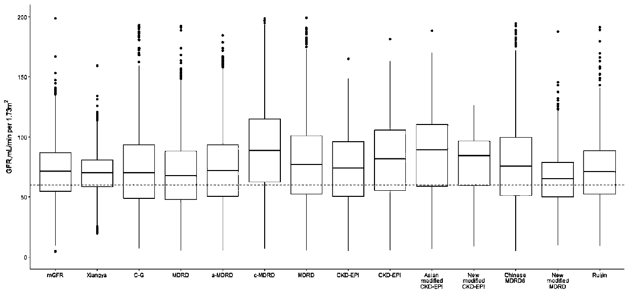
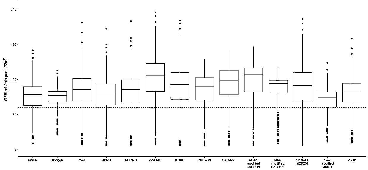
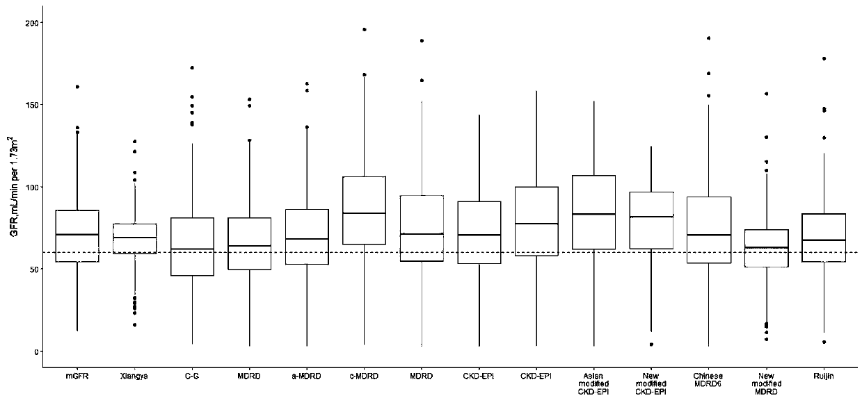
[0376] It should be noted, Figure 1-Figure 5 The horizontal line in the box in the box chart indicates the median; the upper and lower margins of the box indicate the upper and lower quartiles (Q3 and Q1); each of the two ends of the rectangle represents a line segment to the farthest point that is not an outlier , Represents the distribution interval of the normal value of the batch of data, defined as: upper and lower frame margins ± 1.5 × interquartile range; circles indicate abnormal values. The dotted line indicates mGFR=60 as a node. The closer the horizontal line in the box is to the dotted line, the closer the median of the eGFR formula is to the mGFR value, and the more the formula can reflect the true level of GFR.

[0377] Figure 1-Figure 5 It shows a box plot comparing eGFR and mGFR obtained by different functional expressions (including Xiangya formula, existing Chinese or Asian and clinically commonly used creatinine formula) in Chinese populations in different hospitals. The median mGFR of TXH, SXH, and FXH hospital inpatients, TXH outpatients and SXH outpatients were 71.32mL/min/1.73m, respectively 2 , 70.72mL/min/1.73m 2 , 86.70mL/min/1.73m 2 , 77.88mL/min/1.73m 2 And 67.90mL/min/1.73m 2. The median of Xiangya formula is closer to mGFR, and the interquartile range (IQR) is smaller, indicating that its model fitting effect is better than other equations. As shown in Table 5, in the box plot comparing eGFR and mGFR obtained by different functional expressions of inpatients in TXH hospital, the P of inpatients 30 The level of Xiangya equation is the highest at 79.21%, followed by the new and improved MDRD formula (75.08%), reaching P 30 ≥75% of the standard. It is worth noting that when sorting these equations according to accuracy, we found that the Xiangya formula is the first in almost all patient subgroups from the 3 hospitals.

[0378] Table 5 Performance comparison between Xiangya formula and other eGFR formulas in all inpatients included in TXH hospital

[0379]

[0380] In general, the Xiangya formula estimates the eGFR of the Chinese population more accurately than existing formulas.

[0381] This specific embodiment also includes the application of a model for obtaining the glomerular filtration rate of the Chinese population in obtaining the glomerular filtration rate of the Chinese population, the model being established according to the above-mentioned establishment method.

[0382] It should be noted that all analysis results in this specific embodiment adopt R language 3.4.2 (Free Software Foundation, Boston, Massachusetts) and SAS statistical analysis software 9.4 (Statistical Analysis Software Institute, Cary, North Carolina) Calculation.

[0383] Unless otherwise defined, all technical and scientific terms used herein have the same meaning as commonly understood by those skilled in the technical field of the present invention. The terms used in the specification of the present invention herein are only for the purpose of describing specific embodiments, and are not intended to limit the present invention. The technical features of the above-mentioned embodiments can be combined arbitrarily. In order to make the description concise, all possible combinations of the technical features in the above-mentioned embodiments are not described. However, as long as there is no contradiction in the combination of these technical features, All should be considered as the scope of this specification.

[0384] Although the embodiments of the present invention have been described with reference to the accompanying drawings, those skilled in the art can make various modifications and variations without departing from the spirit and scope of the present invention, and such modifications and variations fall under the appended rights. Within the scope defined by the requirements.