

Quadruped robot single-leg trajectory tracking control method and system
A quadruped robot, trajectory tracking technology, applied in general control system, control/adjustment system, adaptive control, etc., to achieve the effect of improving trajectory tracking performance, high-precision trajectory tracking control, and improving performance
- Summary
- Abstract
- Description
- Claims
- Application Information
AI Technical Summary
Problems solved by technology
Method used
Image

Examples
Embodiment 1
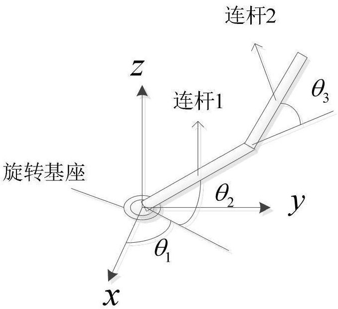
[0035] Such as figure 1 As shown, a quadruped robot single-leg trajectory tracking control method, including:
[0036] Get the joint parameters of the quadruped robot;
[0037] Establish a single-leg dynamic model based on joint parameters;
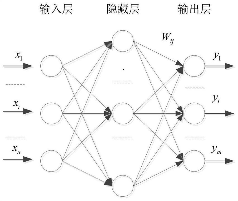
[0038] Correct the single-leg dynamic model based on the disturbance and neural network, construct a single-leg dynamic model considering the disturbance, and assume a reference trajectory;
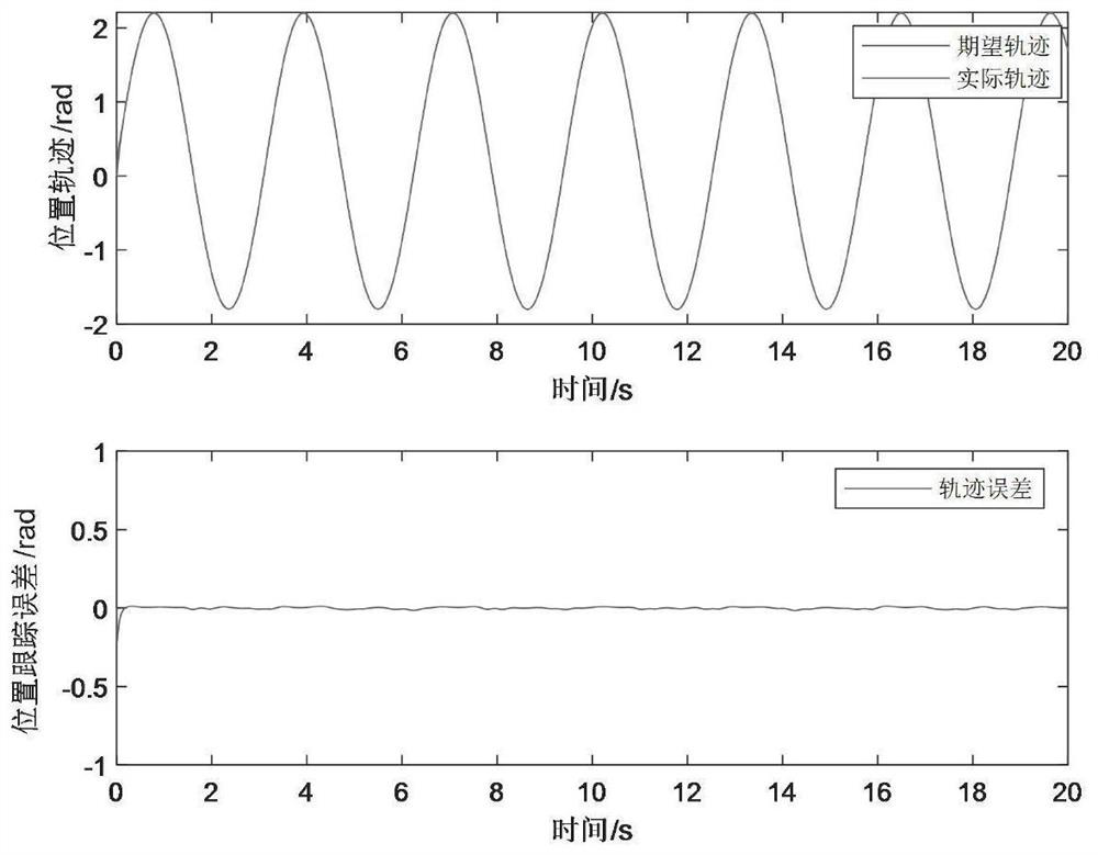
[0039] Use the value function approximation method based on neural network learning to obtain the optimal parameters of the reference trajectory and obtain the optimal control rate;
[0040] Based on the optimal control rate to realize the single-leg trajectory tracking control of quadruped robot.
[0041] Further, the joint parameters include joint positions, velocities and acceleration vectors.
[0042] Further, the establishment of the single-leg dynamic model according to the joint parameters includes obtaining the control moment vector accor...
Embodiment 2
[0118] The present disclosure provides a single-leg trajectory tracking controller for a quadruped robot, including:
[0119] A data acquisition module configured to acquire joint parameters of the quadruped robot;
[0120] A single-leg dynamic model establishment module configured to establish a single-leg dynamic model according to joint parameters;
[0121] The reference trajectory building module is configured to correct the single-leg dynamic model based on the disturbance and the neural network, construct a single-leg dynamic model considering the disturbance, and assume a reference trajectory;
[0122] The control rate acquisition module is configured to use a value function approximation method based on neural network learning to obtain the optimal parameters of the reference trajectory and obtain the optimal control rate;
[0123] The tracking control module is configured to implement single-leg track tracking control of a quadruped robot based on an optimal control ...
Embodiment 3
[0126] The present disclosure provides a single-leg trajectory tracking control system for a quadruped robot, which includes the above-mentioned single-leg trajectory tracking controller for a quadruped robot.
PUM
 Abstract
Description
Claims
Application Information